


Managing Retail Food Waste & Markdowns
Increasing sales and reducing waste in the fresh supply chain
Table of Contents:
- Abstract
- Foreword
- Executive Summary
- Introduction, Background and Purpose
- - Scale of the Problem
- - Impact of Waste on the Shopper and Retailer’s profitability
- - Methodology
- Methodology
- - The Efficient Frontier
- - The Fresh Case Cover
- Key Findings
- - Waste grows exponentially with On Shelf Availability
- - The Fresh Case Cover is a simple and strong first indicator for waste
- - Waste per store varies significantly, due to differences in Fresh Case Cover and due to store replenishment and execution
- Recommendations
- - Find the optimal mix between OSA and %Waste by selecting the sweet spot on the Efficient Frontier
- - Develop strategies to shift the Efficient Frontier
- - Determine how Fresh Case Cover is driving your waste.
- - Benchmark stores and analyse their behaviour
- - Use the 65 point checklist to identify new ideas to reduce waste
- Appendices
- - A: User manual for the “Sell More, Waste Less” tool
- - B. Checklist with improvement suggestions to reduce waste and/or increase sales for the fresh departments
Languages :
This ECR-report shows how retailers can increase their sales, sell fresher products or reduce their food waste. Using data on actual sales and waste for three product categories (convenience products, fruits & vegetables and fresh meat) at 27 selected stores from three retailers in Europe, this report shows that waste is a choice and retailers have several opportunities to increase profit in their fresh supply chains. The two improvement options giving very large reductions in waste are:
• Increasing the product’s shelf life with one day
• Unpacking items in the distribution centre and ship stores smaller quantities
Increasing the product’s shelf life with one day will reduce waste with 42.8% (or increase on-shelf availability with 3.4%), unpacking the items in the distribution centre will reduce waste with 32.5% (or increase on-shelf availability with 2.0%).
To identify which products are the best candidates for increasing the product’s shelf life, decreasing the case pack size or increasing daily sales a very simple indicator has been used, called the Fresh Case Cover. The Fresh Case Cover is simply equal to the ratio of the case pack size and the average daily demand times the product’s shelf life. The actual waste data from the retailers show that the Fresh Case Cover is a strong first indicator for the percentage of waste and hence can be used as a simple means to identify the products with the highest improvement potential. Application of the Fresh Case Cover at Albert in Czech resulted in savings of 1 million euros per year.
Together with this report an Excel-based tool is available (free for ECR-members) which can be used to:
- Increase profit by choosing the right mix between %Waste and On-Shelf-Availability (OSA)
- Quantify and prioritize improvement projects to reduce waste or increase OSA
- Benchmark stores to identify the best-in-class behaviour.
Finally, a check list is available with more than 65 interventions aimed at reducing waste in the retail supply chain, based on interviews and a literature review. It can be used both as a checklist and as an inspiration for retailers to find new ways to reduce waste and increase sales for fresh products.
Abstract
This ECR-report shows how retailers can increase their sales, sell fresher products or reduce their food waste. Using data on actual sales and waste for three product categories (convenience products, fruits & vegetables and fresh meat) at 27 selected stores from three retailers in Europe, this report shows that waste is a choice and retailers have several opportunities to increase profit in their fresh supply chains. The two improvement options giving very large reductions in waste are:
• Increasing the product’s shelf life with one day
• Unpacking items in the distribution centre and ship stores smaller quantities
Increasing the product’s shelf life with one day will reduce waste with 42.8% (or increase on-shelf availability with 3.4%), unpacking the items in the distribution centre will reduce waste with 32.5% (or increase on-shelf availability with 2.0%).
To identify which products are the best candidates for increasing the product’s shelf life, decreasing the case pack size or increasing daily sales a very simple indicator has been used, called the Fresh Case Cover. The Fresh Case Cover is simply equal to the ratio of the case pack size and the average daily demand times the product’s shelf life. The actual waste data from the retailers show that the Fresh Case Cover is a strong first indicator for the percentage of waste and hence can be used as a simple means to identify the products with the highest improvement potential. Application of the Fresh Case Cover at Albert in Czech resulted in savings of 1 million euros per year.
Together with this report an Excel-based tool is available (free for ECR-members) which can be used to:
- Increase profit by choosing the right mix between %Waste and On-Shelf-Availability (OSA)
- Quantify and prioritize improvement projects to reduce waste or increase OSA
- Benchmark stores to identify the best-in-class behaviour.
Finally, a check list is available with more than 65 interventions aimed at reducing waste in the retail supply chain, based on interviews and a literature review. It can be used both as a checklist and as an inspiration for retailers to find new ways to reduce waste and increase sales for fresh products.
Foreword
It is with great pleasure that we are able to present this report – the ECR Community Shrink and On-Shelf Availability Group warmly endorses its findings and urges all retailers to reflect upon the implications and the recommendations of this research for their own organisations.
With a third of all food lost or wasted between the farm and the fork, the problem of food waste has never been more in the spotlight and of more importance to the consumer and the industry. A point underlined in June 2015, when the Consumer Goods Forum (CGF), a network of some 400 retailers and manufacturers made a pledge to halve the food they waste within their own supply chains by 2025.
As Paul Polman, Chief Executive of Unilever stated, “It is a tragedy that up to 2 billion tonnes of food produced around the world is lost or wasted never making it on to a plate. At a time of growing food insecurity and climate change, we can’t afford to let this continue."
Dave Lewis, Group Chief Executive of Tesco further underlined this commitment to change when he declared at the launch of the Champions 12.3 food waste initiative. “At Tesco, we’re committed to tackling food waste not only in our own operations but also through strong and effective partnerships with our suppliers and by helping our customers reduce waste and save money”
In light of this, this report and the research can be seen as very timely, focusing in on specifically what retailers and manufacturers can do together to address the food waste problem within their retail supply chains, and while this in itself may only contribute to 5% of the total food that is wasted, the impact of the changes that can be delivered by implementing the recommendations in this report can be very profound, reducing food waste within the retail supply chain and beyond.
We very much hope that you find this report of interest and if you would like to learn more about the work of the ECR Community Shrink and On-Shelf Availability Group, then we would be delighted to hear from you.
John Fonteijn, Chair,
ECR Community Shrink & OSA Group
www.ecr-shrink-group.com
Royal Ahold
Executive Summary
The ECR Community Shrinkage & On-Shelf Availability Group commissioned Eindhoven University of Technology to deliver important new research that quantifies the relationship between waste and On-Shelf Availability (OSA).
The research results show that
- Waste is a choice,
- Very large reductions in waste (or equivalently: large increases in OSA) are possible,
- Key drivers of waste are the OSA target level, the case pack size, the shelf life, the average daily demand per item-store combination and finally store replenishment and execution.
This research project provides the ECR-members with new facts and tools to find the optimal mix between waste and OSA, to benchmark fresh departments in stores in a fair way, to quantify the improvement potential and to generate new interventions.
Often retailers view waste as a fact of life. Actually, the research results show that waste is a choice and retailers have several opportunities to increase profit in their fresh supply chains.
Three improvement options delivering a large reduction in waste are:
- To increase the product’s shelf life with one day
- To unpack items in the distribution centre and ship stores smaller quantities
- To differentiate target OSA levels for slow-moving items and fast-moving items
Existing models to approximate waste and OSA have been used to quantify the benefits when these three improvement options would be applied to three product categories (convenience products, fruits & vegetables and fresh meat) at 27 selected stores from three large supermarket chains in Europe participating in this project. When applying these models, using empirical data from 17,093 item-store combinations as their input, the three improvement options will have the following benefits:
Increasing the product’s shelf life with one day will reduce waste by 42.8% (or increase on-shelf availability by 3.4%), unpacking the items in the distribution centre will reduce waste by 32.5% (or increase on-shelf availability by 2.0%) and differentiating target OSA levels for slow-moving items and fast-moving items will reduce waste by 12.0% (or increase on-shelf availability by 1.3%). The improvement potential for these options as well as their ranking differs per retailer. Still, for each retailer large benefits can be achieved from these improvement options.
To identify which products are the best candidates for increasing the product’s shelf life, decreasing the case pack size or increasing daily sales, a very simple indicator has been used, called the Fresh Case Cover. The Fresh Case Cover is simply equal to the ratio of the case pack size and the average daily demand multiplied by the product’s shelf life. The actual waste data from the retailers show that the Fresh Case Cover is a strong first indicator for the percentage of waste and hence can be used as a simple means to identify the products with the highest improvement potential.
When comparing the performance of different stores, a large variation of waste is observed. A substantial part of this variation is caused by the variability in daily sales, case pack sizes and shelf lives between stores. But even when controlling for those factors, it is observed that stores still have large variations in waste. This remaining variation in waste is likely due to store replenishment and execution, i.e. the procedures and procedure compliance in stores as well as the system or logic which is used to replenish the inventories in the stores. Store replenishment and execution can be improved for example, by giving the right information, training and incentives to the store managers, engaging the employees who replenish the shelves, rotating correctly and by making the right replenishment decisions.
The improvement potential to reduce waste and increase product freshness is different per retail chain, per store and per product category. For example the five stores with the highest improvement potential have approximately 72% more waste compared with their benchmark, while the five stores with the lowest improvement potential only have 17% more waste compared with their benchmark. These percentages are the maximum values for the potential waste reduction per store since the benchmark does not take into account all factors causing waste. The results also show that for stores with relatively low average demand the focus should be on improving the supply chain (e.g. by shipping smaller quantities to the stores or increasing the shelf life), while for stores with relatively high average demand the focus should be on improving the store replenishment and execution.
To assist retailers and their suppliers in their struggle to improve the performance of the fresh supply chain a new tool is made available, called the “Sell More, Waste Less” tool. It is a simplified version of the benchmarking tool used throughout this research project. This benchmarking tool was already available before the “Sell More, Waste Less” project and is based on recent scientific results to quantify waste and on shelf availability as a function of key product and demand characteristics (like shelf life, case pack size and average daily demand). The tool can be used by retailers and their suppliers to:
- Increase profit by choosing the right mix between %Waste and OSA
- Quantify and prioritize improvement projects to reduce waste
- Benchmark stores to identify the best-in-class behaviour
The “Sell More, Waste Less” tool developed in this project is simple to use (Excel-based) and makes a fair comparison between stores and/or categories. With this tool retailers are able to identify which stores and which fresh departments have the biggest gap between the actual performance and the benchmark. The output of this gap-analysis can act as a starting point for a discussion with store managers on best practices. Moreover, analysing per store a small sample of item-store combinations with the largest and the smallest gaps, has proven to be a very efficient and effective way to identify the reasons why fresh departments outperform or underperform.
In addition to the benchmark tool, a check list is created with 65 interventions aimed at reducing waste in the retail supply chain, based on interviews and a literature review. It can be used both as a checklist and as an inspiration for retailers to find new ways to reduce waste and increase sales for fresh products.
Introduction, Background and Purpose
Customers entering a hypermarket in Europe today see a mouth-watering display of fresh food. The abundance and breadth of assortment reflect the desire of shoppers for choice and freshness. But the excessive supply required to sustain this constant availability across a full range of choice can come with a price: high levels of food waste. Retailers are faced with the costs and social stigma of waste and look for ways to deal with the trade-off between availability and waste.
The ECR Community Shrinkage and On-Shelf Availability Group commissioned Eindhoven University of Technology to firstly deliver important new research results that quantify the relationship between waste and OSA (On-Shelf Availability) based on empirical data. Secondly, they asked the researchers to create and bring to their members practical tools and techniques that could help them better manage the balance between waste and OSA. Finally, the researchers were asked to prepare a checklist with improvement suggestions.
In the last ten years, the Eindhoven University of Technology has developed and published a coherent set of research results for perishable items, including a new replenishment logic specifically developed for perishable items in supermarkets, mathematical expressions which quantify both onshelf availability and waste as a function of key product and demand characteristics and an Excelbased tool to set replenishment parameters and to determine Key Performance Indicators for perishable items.
In this “Sell More, Waste Less” project, these previous results are further validated using the empirical data from the three participating supermarket chains. In addition, during this project the research results were also improved and made more robust where needed (for example by developing new theory for situations with very large waste) and a simplified version of the Excel-based tool has been developed, which is easy to use for practitioners. All the results of this project will enable practitioners to quantify their improvement potential and to pull the right levers to influence their own organisations performance on waste and OSA.
One of the purposes of this research project is to illustrate to retailers that waste is not a given, but a choice. Quantitative analyses will demonstrate that the waste level heavily depends on decisions made throughout the retail supply chain and that by making appropriate decisions the current waste levels can be reduced to a large extent, having a huge potential impact on the retailer’s profitability and market share.
In addition, improvement suggestions are gathered from several sources, with the purpose to inspire managers and employees throughout the retailer supply chain to create new ways of working and help the company to reduce waste and help their consumers to get excited about really fresh products.
Scale of the Problem
Roughly one-third of food produced for human consumption is lost or wasted globally, which amounts to about 1.3 billion tons per year, according to Gustavsson et al. (2011). The associated costs are estimated to be equal to 856 billion euro’s each year (WRAP, 2015). The percentage of waste at the retail level reported in the literature varies considerably, both between product categories and between countries. Waste (as a percentage of aggregated sales) varies for example between 4% for meat and 11% for dairy products in the USA (Buzby et al., 2014). For Fruit & Vegetables for example, waste is reported to be 8-9% of volume of sales in Switzerland and 9% of food supply value in the USA, while studies in Sweden, Norway and Austria report waste in the range of 4%-5% (Sweden 4.3% of delivered quantity (mass), Norway 5.1% of total turnover and Austria 4.3% of sales in cost price; see Table 8 in Lebersorger and Schneider, 2014). The variation at the item level is even larger. Buzby et al. (2015) show for a selection of 55 Fruit and Vegetables items that total shrinkage (defined as a percentage of the weight that arrives at the stores) at five US retailers varies between 2.2% for sweet corn and 4.1% for bananas to 43.1% for papayas and 62.9% for turnip greens. While all these numbers suggest that waste at the retail level is significant, in this report we will not primarily focus on the level of waste but we rather focus on the improvement opportunities: how much can waste at the retail level be decreased and how?
Impact of Waste on the Shopper and Retailer’s profitability
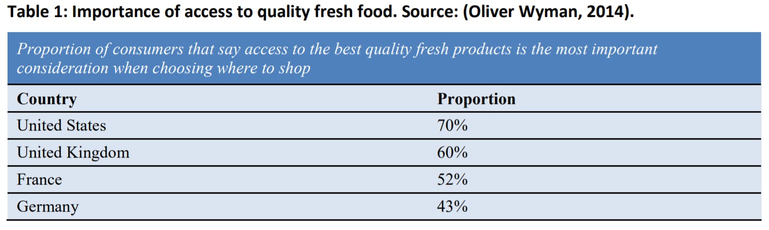
As reported by Gustavsson et al. (2011), while waste at the retailer is significant, especially in developed regions like Europe and the USA even more food is wasted at the final consumer level. This implies a multiple-win effect for retailers: If retailers reduce waste and thereby increase the remaining product’s shelf life available for consumers, their actions may not only reduce their own operational costs and waste, but also help to reduce the waste at the consumer level and at the same time increase the product freshness experienced by the final consumers. Lütke Entrup (2006) argues that product freshness is one of the most important buying criteria for consumers. This is supported by more recent numbers from Oliver Wyman (2014), a global management consultancy with a practice in food waste, and reported in Table 1. So the retailer who succeeds best in improving product freshness may not only reduce costs due to waste and increase its social responsibility image, but may also increase its market share.
The financial potential for retailers is huge. If the average percentage of food waste (some benchmarks suggest that food waste can be 2% of total sales value) can be reduced by just 0.5% point (e.g. reducing waste from 2% to 1.5% of the retailer’s total sales value), a typical retailer having a net income margin of 3% can increase its net income by 17%. In this report multiple options will be presented which can lead to waste reductions of 25% or even more.
Structure of the report
The report is organised as follows: In Section 2 a description is given of the methodology, the research environment and the data which have been collected and analysed. Next, the tool which has been used throughout this research project to estimate waste and On-Shelf Availability is introduced and finally two key concepts are introduced which are very helpful in exploring and explaining the potential to reduce waste. These two concepts are the Fresh Case Cover and the Efficient Frontier. In Section 3 the results of this project are presented: first it is shown that a trade-off exists between OSA and waste, next it is shown that waste can be explained to a large extent by the Fresh Case Cover and third it is shown there are large variances in the performance of different stores, which can be explained by the Fresh Case Cover and by the store replenishment and execution. In Section 4 the results are translated into recommendations for retailers and their suppliers. Finally, in Section 5 the limitations are discussed and suggestions for future research are provided.
Methodology
In section 2.1 we will describe the methodology applied, the research environment, the data gathered and the data issues which have been resolved. Section 2.2 will describe the tool which is used throughout this research project to evaluate the performance of the retailers and to quantify the improvement potential of waste reduction projects. In Section 2.3 two key concepts are introduced which will help to explain the results: the Fresh Case Cover and the Efficient Frontier.
The methodology, research environment and data
Methodology
For this report different research methods have been applied. For the benchmarking of the 27 supermarkets who participated in this research project, for the quantification of the improvement opportunities and for prioritising the improvement projects, empirical data was collected from the participating retailers and a benchmarking tool used.
Note, this benchmarking tool already existed before the “Sell More, Waste Less” project started and is based on scientific results which have been published in scientific journals over the last decade. These scientific results include a new replenishment logic for perishable items (Broekmeulen and Van Donselaar, 2009) and mathematical expressions for the service level (OSA) and the percentage of waste as a function of key product and demand characteristics (Van Donselaar and Broekmeulen, 2012 and 2013).
For best practices, these have been collected using interviews with retailers, the experience gathered from executing master thesis projects with retailers and by reviewing the available literature
Description of participating retailers, available data and data issues
Three large European Grocery retailers participated in this research. The supermarkets all carried large assortments. For this research project, nine stores were selected per retailer; three small, three medium and three large stores from the supermarket store format. It should be stressed that the retailers carry multiple store formats (from convenience stores to hypermarkets and e-commerce) and the sample of nine stores do not represent all their store formats. As a consequence, the results from this research project cannot simply be extrapolated to the aggregate retail company level.
The research focussed on three product categories: convenience, fruits and vegetables and meat. According to (WRAP, 2015), these three categories are responsible for about 50% of the waste. Note that the three retailers have different definitions for the three product categories. For example, burgers are classified as convenience by one retailer and as fresh meat by another retailer.
In the “Request for Data”, retailers were asked for items that are sold in consumer units and not in kilograms (weight), to avoid issues with the sales amount and the exact amount in a case pack. The sample was also limited to products that are supplied to the store from the retailer’s distribution centre. In this way the lead time and the average product’s shelf life that the stores received were controlled. This had an effect on the considered assortments since the retailers differ in which part of their assortment is delivered from their distribution centre or directly from the supplier. Therefore, the focus in this research project will be on comparing the performance of the 27 stores and comparing the performance of the three product categories rather than on comparing the three retailers for each product category.
For every item-store combination the retailers provided the following data on a confidential basis: the case pack size, the store shelf life (i.e. the product’s shelf life on the moment the product enters the store) and daily sales, waste and supply (i.e. deliveries to the store) data. The daily data were provided over the period 2013-2015. Exact starting and end dates for these daily data differed somewhat per retailer, but each retailer provided data during at least one full year in the time-frame 2013-2015.
To reduce issues with products that are phasing in and/or phasing-out of the assortment, the assortment was further limited to item-store combinations that had at least three deliveries and three weeks of sales during one year. The resulting total number of items in the database is equal to 2474: 1044 convenience items, 820 fruits and vegetables and 610 meat items.
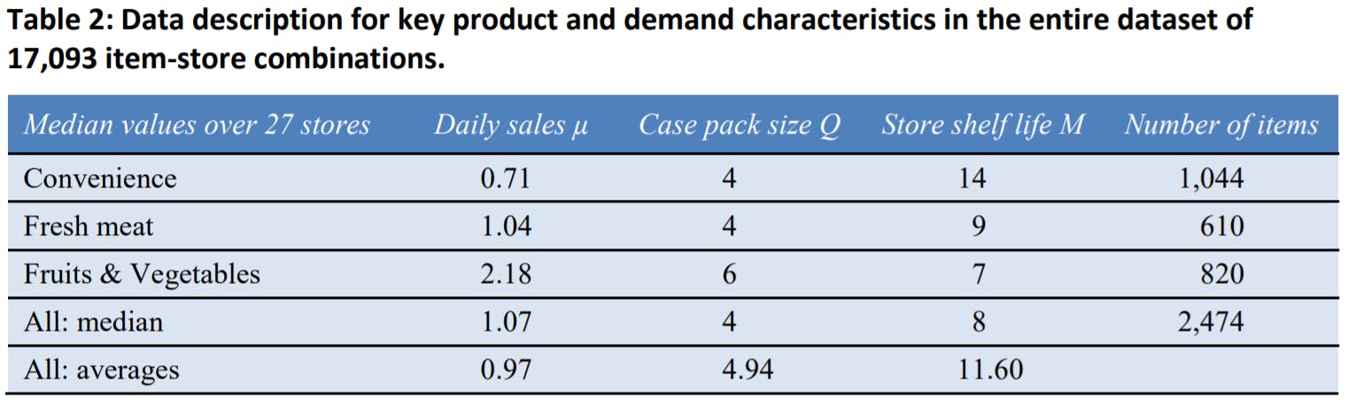
The first three rows in Table 2 show for each of the three product categories the median values of the daily sales, the case pack size and the store shelf life of all item-store combinations in the entire database which belong to the specific category. The fourth column shows the number of items in each product category. The fourth row shows the median value of the daily sales, the case pack size and the store shelf life based on all 17,093 item-store combinations in the entire database, resulting from the 2474 items and the 27 stores selected. While the fourth row reports the median values, the last row reports the average values of the daily sales, the case pack size and the store shelf life based on all 17,093 item-store combinations.
The reported sales is the regular sales, excluding promotions. For the retailers that did not register the promotions in the point of sale data, these were determined from the level of price reduction (at least 15%) and/or the lift factor (at least 3) compared to the base sales level before and after the promotion period. The promotion period was typically a week, but the starting weekday of a promotion week depends on the retailer.
The reported waste includes discounted items close to the expiration date, measured in consumer units. If a retailer did not register the waste in consumer units but in sales value, the waste was estimated using the average regular price three weeks before and after the time of waste registration.
The actual waste percentage is calculated relative to the sales (both waste and sales are in number of consumer units):
%Waste = 100%*(Waste/Sales)
An alternative measure would be to calculate the waste relative to the supply, but significant mismatches were encountered between registered inflow and registered outflow per item-store combination. These mismatches can be due to many reasons, e.g. theft, damage, errors in delivering, errors in scanning, in store use, errors in the actual case pack sizes and/or changes in the case pack size during the year.
2.2. The benchmarking tool
A benchmarking tool has been used throughout this research project to evaluate the performance of the retailers. The tool can also be used to assist retailers in reducing waste. The tool can be used for example to support the retailers to:
- Benchmark stores within a retail chain
- Increase profit by choosing the right mix between %Waste and On Shelf Availability (OSA)
- Prioritise improvement projects to reduce waste
Below the input, the output, the logic and assumptions behind the benchmarking tool as well as the limitations will be described. Based on the logic of the benchmarking tool used in this research project, an easy-to-use Excel-based tool called the “Sell More, Waste Less” tool is created for retailers and their suppliers. The “Sell More, Waste less” tool essentially is a simplified version of the benchmarking tool. For details on this tool we refer to the short user manual which is provided together with the tool. This “Sell More, Waste Less” tool and the short manual are disseminated for free via the website of the ECR Working Group Shrinkage and On-Shelf Availability: www.ecrshrink-group.com.
The input needed in the benchmarking tool is the lead time and the review period for the supermarkets, together with the average daily demand, the case pack size, the average store shelf life and the reorder level (or alternatively the target OSA) for one item-store combination (or for a set of item-store combinations if the tool is used to benchmark fresh departments or stores).
- The lead time is the time between the moment of ordering by the store and the moment the replenishment order is stacked on the shelf
- The review period is the time between two moments when the store reviews the inventories for a group of items which are delivered simultaneously and decides on the replenishment quantities for each of these items. The review period is typically equal to the time between two moments when the retailer’s distribution centre delivers this group of items to the store
Example: Imagine a store with a product category which is delivered by the DC once every day. Then the items in this product category for this store have a review period equal to one day. If for this store the replenishment order which is created on Tuesday at 21.00 pm gets delivered to the store and stacked on the shelf on Wednesday 21.00 pm, then the lead time for this store is equal to one day.
In this research project as well as in the “Sell More, Waste Less” tool both the lead time and the review period are set equal to one day, based on interviews with the retailers.
- The average daily demand (per item per store) is estimated from the sales data in regular (nonpromotion) weeks when the item is part of the store’s assortment; if the On Shelf Availability (OSA, also known as the fill rate) is large the average daily demand can indeed be approximated by the average daily sales
- The case pack size is equal to the base quantity in which an item has to be ordered by a store. For example, if strawberries are always supplied in plastic crates containing 6 consumer units (a consumer unit is for example a carton box containing 500 grams strawberries) and the store has to order in (integer numbers of) full crates, the case pack size is 6 consumer units.
- The store shelf life of an item is the average time between the expiration date and the moment the item arrives in the supermarket
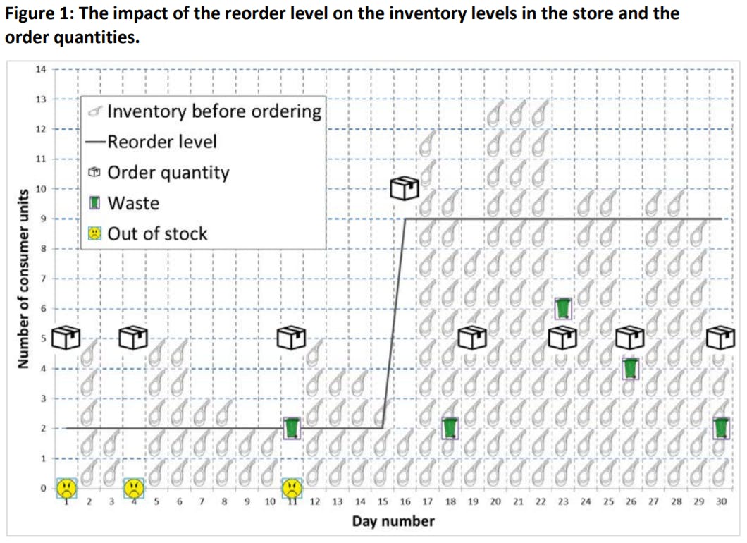
- The reorder level (also known as the reorder point) is the inventory level which triggers a replenishment of the inventory for an item in the store: when (at a review moment, which in most stores with sales based ordering systems is set at once a day) the inventory level falls below this reorder level, a new replenishment order is created. So the lower the reorder level, the lower the inventory level will be at the moment a new order is created. This lower inventory level can imply a lower OSA, and also a lower waste
Example: Imagine a product with a lead time equal to one day, a review period equal to one day, a case pack size equal to 5 consumer units, a shelf life equal to 6 days and an average daily demand equal to 1 consumer unit/day. Figure 1 shows for this product how the reorder level affects the quantity ordered, the inventory in the store just before a replenishment decision is made, the number of out-of-stocks and the amount of waste. The impact of the reorder level becomes particularly evident when it is raised; from day 16 on the reorder level is raised from 2 consumer units to 9 consumer units. Every day the minimal number of case packs is ordered which is required to bring the inventory position for this product to be at or above the reorder level. So the order quantity on a given day is only positive if the inventory before ordering on that day is strictly below the reorder level. In the first part of the graph (Figure 1) the inventories are very low due to the low reorder level and as a result the store is frequently out of stock (i.e. when inventory before ordering is equal to zero), while in the second part of the graph the inventories are very high and hence the store is never out of stock. On the other hand, waste will be low in the first part of the graph and high in the second part of the graph.
In this research project, the retailers did not provide their reorder levels, but instead they provided in interviews their target OSA levels. Based on these target OSA levels the reorder levels were determined for every item-store combination in the database using the inverse logic of the benchmarking tool.
The output of the benchmarking tool consists of approximations for several Key Performance Indicators (KPI’s) of the inventory system. The tool provides five KPI’s:
- The On-Shelf Availability (OSA) is the percentage of customer demand delivered from the shelf;
- The waste percentage (%Waste) is the total waste per period as a percentage of total demand in the same period. Both waste and demand are measured in consumer units (CU’s );
- The freshness to customer is the average number of remaining shelf life in days for the customer (from the moment the customer buys the product till the expiration date);
- The number of order lines is the average number of order lines per review period. This represents the probability that at a review moment the item-store combination is ordered
Example: Imagine a store where the inventories are reviewed once every two days and where a certain itemstore combination based on daily sales is ordered once every 10 days. This implies that this item-store combination will be ordered once in every five review moments and hence the number of order lines per review moment is 1/5=0.2.
- The probability non-empty shelf is the probability that the shelf for this item is not empty just before a new delivery is made for this item or for another item in its category (i.e. when the store looks most empty);
These KPI’s can be used for example to evaluate the impact of the key drivers on waste, to evaluate cost functions for different improvement projects, to benchmark the performance of individual stores and to evaluate a new product introduction. Alternatively, if only a target OSA is known (and no cost data are available), the benchmarking tool can provide as its output the reorder level which is needed to reach this target OSA and based on this reorder level it provides the resulting waste, freshness to customer, number of order lines and the probability non-empty shelf.
The logic behind the benchmarking-tool is based on recently developed scientific results for perishables. The mathematical expressions used in the benchmarking tool to calculate the waste percentage and the On Shelf Availability for example are based on approximations published in (Van Donselaar and Broekmeulen, 2012) and (Van Donselaar and Broekmeulen, 2013). The approximation for the waste percentage is a linear function of seven constructs of variables. The linear coefficients in this function are determined using linear regression and are based on results from more than 15,000 simulation experiments. One of the assumptions in the publication on the waste approximation is that the percentage of waste is always less than 30%. Analysis of the empirical data for the three retailers in this research project showed that this assumption is not always met in practice. To deal with this a new approximation has been derived and tested for item-store combinations having more than 30% waste. This new approximation has been included in the latest version of the benchmarking tool.
The approximations for %Waste and OSA which have been developed in the literature all depend not only on the average daily demand but also on the demand uncertainty. To increase the robustness of our approximations, the demand uncertainty was estimated in another way, as suggested in (Silver et al., 1998, p.126). Using linear regression on weekly demand data for a subset of the total database (with items being in the store’s assortment for at least 50 weeks and after excluding the promotions) a relationship was found between the average and standard deviation of the weekly demand. This relationship was transformed into the following simple relationship between the estimated standard deviation of the daily demand and the average daily demand:
𝜎𝜎 = 1.18 ∙ 𝜇𝜇0.77
With
𝜎𝜎 = the standard deviation of the daily demand
𝜇𝜇 = the average daily demand
This method provided robust results. As an additional advantage of this method, the standard deviation no longer has to be measured by the retailer. Instead the benchmarking tool, as well as the “Sell More, Waste Less” tool derived from it, now only needs the average daily demand per itemstore combination as input. This makes the tool also easier to understand and to apply.
The benchmarking tool was also used to evaluate the impact of some key drivers on waste. The logic in the benchmarking tool is based on the assumption of an “ideal world”. In this ideal world a smart replenishment logic is used which takes into account the expected amount of waste when a new replenishment order is generated. If for example in a store the shelf for one item contains eight readyto-eat meals which all expire soon after the replenishment order is made (for example expire the next day), the new replenishment order will take this into account and will already order new products before the old products actually expire. The automated store ordering systems currently in use by retailers do not take this into account and only start ordering new products one review period later, i.e. after the products actually expired and are registered as “waste”. This causes an empty shelf from the moment the goods expire till the new products arrive, while in the smart replenishment logic the new products arrive the moment the old products expire. This replenishment logic is called the Estimated Withdrawal and Aging (EWA) logic and often results in less waste compared with the traditional replenishment logic (Broekmeulen and Van Donselaar, 2009). For retailers who already discount products at the end of the day preceding their expiration date, the number of discounted products is all the extra information which is needed to upgrade their current replenishment systems (assuming the lead time and the review period of the retailer are equal to one day).
In the ideal world it is also assumed that consumers apply the First In First Out (FIFO) withdrawal logic, i.e. they will buy the oldest items from the shelf. Retailers sometimes enforce this behaviour, for example by putting the fresher items behind the older items on the shelf, by having only one or two different ages on the shelf or by physically lowering the distance between shelves making it more difficult for the consumer to look for the freshest items. In practice typically a mix of consumers exist. Some consumers have plenty of time to check all items on the shelf and consider it important to get the freshest items, others do not have this time or simply trust the supermarket based on experience that the oldest item on the shelf is always sufficiently fresh for their purpose. Clearly the percentage of waste is considerably higher when all consumers buy only the freshest items on the shelf (Broekmeulen and Van Donselaar, 2009). However, if a relatively large part of the consumers still trust the supermarket and buy the oldest item on the shelf, the effect on the percentage of waste is limited (compared with the situation that all consumers buy the oldest item on the shelf).
As a base scenario the target OSA is set the same for all items in a store belonging to the same retail chain. When considering the improvement projects later on in this document the impact of using different target OSA levels for different products will be investigated. Retailers use different ways to register the shelf life in their operational databases. If a retailer only registers the minimal store shelf life, it is assumed that the average store shelf life is equal to this minimal shelf life plus one day. According to Tromp et al. (2012) fixed expiration dates are set at a rather cautious level.
There are two limitations to the method applied in this research project. First average sales are assumed to be constant throughout the week, while in reality many retailers are facing an uneven pattern in sales with high sales on Friday and/or Saturday and lower sales on Sunday and Monday. The error due to neglecting this weekly pattern is limited for a number of reasons. The first reason is the fact that many consumers appreciate it when these items are as fresh as possible and some of these consumers are willing to visit the store multiple times a week to get really fresh items. Next, simulation studies have demonstrated that the effect of the weekly pattern on the average percentage of waste is limited compared to the situation when demand is assumed to be stationary throughout the week (Broekmeulen and Van Donselaar, 2009).
The second limitation is the fact that the effect of price discounts (when the products near their expiration date) on sales rate are not included. On the one hand it is likely that the sales rate decreases when the products near their expiration date since consumers prefer fresher items. On the other hand, it is likely that a price discount attracts extra buyers. It is assumed that these two effects neutralize each other and as a result it is assumed that the sales rate is independent on whether or not the price is discounted when the products near their expiration date. Little scientific evidence is available on these discount effects. Even supermarket chains have different views and different strategies with respect to this topic. Some supermarkets discount when fresh products reach their expiration date, while competing supermarkets in the same sales geography do not discount at all, but rather take all items off the shelves one day before the expiration day.
2.3. Two key concepts helping to explain the waste reduction potential
In order to be able to better understand the results from this research project, two key concepts will be explained first. These key concepts are called:
- The Efficient Frontier and
- The Fresh Case Cover.
These two key concepts are based on the main drivers of waste and hence they will prove to be very helpful in exploring and explaining the potential to reduce waste.
The Efficient Frontier
One of the most important drivers for waste is the target On Shelf Availability (OSA) set by retailers. Most retailers are aware that if they increase the target OSA for perishable products, the safety stock (or the reorder levels) used in their inventory replenishment systems will increase. As a result, the inventories on the shelves will increase which finally results in more waste. Few people however know the exact relationship between OSA and %Waste, so they cannot answer questions like “if the target OSA is increased by 2%, how much more waste will this give?” and vice versa. The reason for this is that the percentage of waste not only depends on the target OSA. The percentage of waste is a more complex function which also depends on factors like the average daily demand, the case pack size and the shelf life of the products in their assortment.
To study the impact of the target OSA on %Waste, the so-called Efficient Frontier will be determined. This is the relationship between OSA and %Waste in the ideal world described earlier. It can be interpreted as the minimal %Waste a retailer can achieve for any given OSA. In real life the world is less ideal and so more waste will be realised than the waste represented in the Efficient Frontier. The benchmarking tool, explained earlier in this report, is used to determine the Efficient Frontier, based on empirical input data provided by the retailers. The Efficient Frontier can be determined per itemstore combination or for a set of item-store combinations.
Example: To illustrate how the Efficient Frontier is determined for a single item-store combination, consider the fictitious example of a tray of 4 Braeburn apples sold in a store in Liverpool. In this store these apples sell on average 1 consumer unit (=1 tray) per 2 days, so the average daily demand is 0.5 consumer units. These apples can be ordered by the store in crates containing 4 trays (x 4 apples) and the shelf life is equal to 11 days. With this input data the benchmarking tool calculates for every possible reorder level the resulting OSA and %Waste in an ideal world. Table 3 shows the results from the benchmarking tool for this item-store combination:

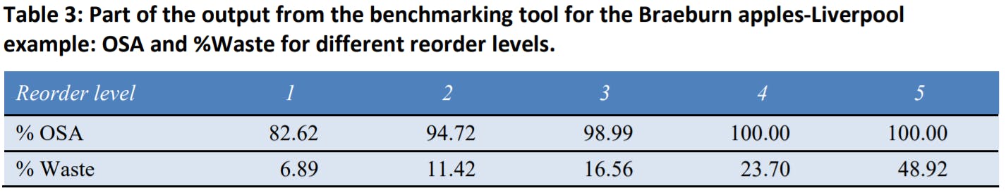
So when for example a reorder level equal to 2 consumer units is used in the inventory replenishment system, the resulting OSA is equal to 94.72% and the %Waste is equal to 11.42%. As explained in the example in Section 2.2 (see Figure 1) as the reorder level increases, the inventory in the store increases and as a result both the %OSA and the %Waste increase too. This can also be observed in Table 3. When combining the results from Table 3 in a single graph, the Efficient Frontier for the Braeburn apples-Liverpool combination is obtained, see Figure 2.
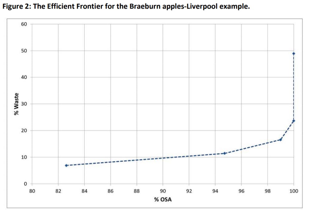
Similar logic is used to determine the Efficient Frontier for a set of item-store combinations. For such a set, multiple target OSA levels are set (ranging e.g. from 85% to 99% in steps of 0.5%). Then for each OSA target level and for each item-store combination in the set the lowest reorder level is determined (using the mathematical expressions in the benchmarking tool) which will provide an OSA equal to at least the target OSA level. For this reorder level both the %Waste and the actual OSA will be calculated. Note the actual OSA may be larger than the target OSA, since reorder levels are discrete numbers (see e.g. Table 3 in the previous example with Braeburn apples in Liverpool: if the target OSA is equal to 93%, the first reorder level reaching or exceeding this 93% is equal to 2 consumer units and the resulting OSA is 94.72%). Finally the %Waste and the OSA for the entire set of item-store combinations is determined by taking the weighted %Waste and the weighted OSA of all item-store combinations, using the average daily demand as the weight factors.
The Fresh Case Cover
Key drivers, other than the OSA, having a direct impact on the amount of waste are the shelf life (m), the average daily demand (μ) and the case pack size (Q). Before analysing one by one the effects of the shelf life, the average daily demand and the case pack size on waste using the benchmarking tool in an ideal world, first the combined effect of these three key drivers of waste will be analysed in the real world, i.e. based on actual waste data and product data from the retailers. Hereto the concept called the Fresh Case Cover (FCC) is introduced. The Fresh Case Cover is simply equal to the case pack size divided by the average demand during the shelf life. So we have
A similar measure, the inverse of this ratio, has been used in a publication analysing the waste for meat and dairy products in Sweden (Eriksson, 2014). Since the ratio 𝑄𝑄⁄𝜇𝜇 is known as the case pack cover (Van Donselaar et al., 2010), we refer to the ratio 𝑄𝑄⁄(𝑚𝑚 ∙ 𝜇𝜇) as the Fresh Case Cover (FCC).
If demand were constant and known beforehand, then waste only occurs if demand during the shelf life is less than the case pack size, i.e. 𝑚𝑚 ∙ 𝜇𝜇 < 𝑄𝑄. So then waste only occurs if FCC>1. If for example for an item the case pack size is equal to 6 consumer units, the demand is 2 consumer units per day and the shelf life is equal to 3 days (so FCC=1), then the case pack is sold just before the products expire and as a result no waste occurs. As soon as the demand per day is less than 2 consumer units per day (i.e. FCC>1), then the case pack can no longer be sold completely during the shelf life and one or more consumer units will be wasted.
Note that if in this same example demand is uncertain, waste will occur even though the average daily demand is still 6 consumer units and FCC=1. To see this, consider the same example but now with demand during three days being equal to 4 consumer units with a probability of 50% and equal to 8 consumer units with a probability of 50%. Then with a 50% probability the waste is equal to (6 - 4=) 2 consumer units and a 50% probability that waste will be zero. So the average waste is now equal to 50%*2 + 50%*0 = 1 consumer unit. Even more waste will occur if the retailer also adds a safety stock to buffer against the demand uncertainty. So in the real world where demand is uncertain waste already occurs if 𝐹𝐹𝐹𝐹𝐹𝐹 ≤ 1. Nevertheless, in a world with uncertain demand, FCC remains a very strong metric to predict the amount of waste, as we will see in the Results section.
Key Findings
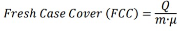
Waste grows exponentially with On Shelf Availability
Based on the empirical data from the three participating retailers and using the benchmarking tool, the Efficient Frontier is determined for the entire dataset (i.e. the set of 17,093 item store combinations). This Efficient Frontier represents the minimal waste (achieved in an ideal world) which can be reached for any given OSA level and is shown in Figure 3. If for example all three retailers would aim for an OSA equal to 95%, the resulting %Waste would be 2.6%. It is clear from Figure 3 that %Waste increases exponentially when OSA increases. This illustrates the importance to determine the right level for OSA. This is not a decision to be left to the designer of an automated store ordering system or a local store department manager who is new in his job, but a strategic decision to be made by topmanagement. The next Section will further elaborate on how top-management can be supported in finding the right mix between the OSA level and %Waste.
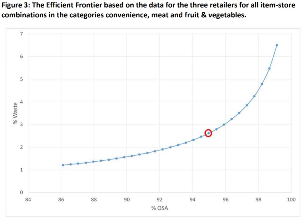
When the Efficient Frontier is determined for each of the three product categories separately (Figure 4), it turns out that the Efficient Frontier for Fruits & Vegetables (the yellow line in Figure 4) is much more efficient than the Efficient Frontier for Fresh Meat (the grey line) and for Convenience (the red line). If for example, the target OSA is equal to 95%, the %Waste for fruit & vegetables is equal to 2%, while for Fresh Meat this is equal to 3.8%. An important contributor to the higher efficiency for Fruits & Vegetables is the fact that their median daily sales per item-store combination is more than twice as large as for the other two product categories (see Table 2). Efficient Frontiers are not only different for different product categories, they are also different for different stores within the same retail chain: large stores having high sales numbers per item typically have Efficient Frontiers which outperform the Efficient Frontiers for small stores with low sales numbers per item.
The Fresh Case Cover is a simple and strong first indicator for waste
The Fresh Case Cover (FCC) introduced in Section 2 turns out to be a strong first indicator for waste. This can be seen from Figure 5, which shows how %Waste depends on the Fresh Case Cover (FCC) for the 27 participating supermarkets. Each point in Figure 5 represents the average actual waste reported by the retailers for the subset of item-store combinations in the total database having a similar value for FCC. Let us take for example the point with FCC=0.5 in Figure 5. For this point from the total database of 17,093 item-store combinations, all item-store combinations are selected which have a value for FCC between 0.45 and 0.5. For these 603 selected item-store combinations both the average waste and the average daily sales are summed up. The ratio of the total average waste for this subset divided by the total average daily sales is the %Waste reported in Figure 5 for the point with FCC=0.5. The other points in Figure 5 are derived in a similar way.
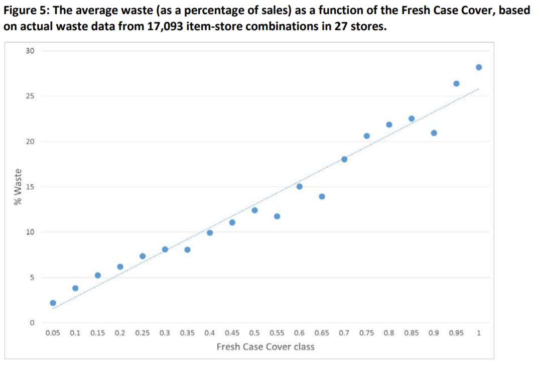
Figure 5 shows there is almost a linear relationship between %Waste and the FCC. This fact combined with the fact that the ratio FCC is extremely simple to calculate, implies that FCC is a powerful first indicator for the %Waste of an item-store combination.
Note however that each observation in Figure 5 represents the average waste for a large subset of item-store combinations (one observation may represent the average waste for a subset containing thousands of item-store combinations); for any individual store-item combination the %Waste not merely depends on the FCC only; it also depends on the exact values for the case pack size Q, the shelf life m, the average daily demand μ and the On Shelf Availability and finally the value is also due to some randomness (since demand is uncertain, waste during one year is also uncertain). This implies that while the FCC is a very strong first indicator for waste when applied to a large set of item-store combinations, the actual waste for one specific item-store combination will show more variation than suggested by Figure 5. This fact is supported when applying linear regression on the relationship between FCC and the actual waste percentage for all 17,093 item-store combinations. The resulting 𝑅𝑅2 is 0.42, which implies that 42% of the variation in the waste percentage is explained by the FCC score. In other words, the FCC score explains a large part of the waste percentage but there are likely also other factors driving the waste percentage that are not measured in this model yet. Also note that the exact slope and intercept in Figure 5 may differ somewhat between different retailers or between different product categories, for example if they have different delivery frequencies from their DC’s to the stores and/or different targets for OSA.
Still any retailer can determine the relationship between the actual %Waste and FCC for their itemstore combinations and use this graph as a simple means to explain to their suppliers or their employees the kind of impact their decisions on the case pack size, the shelf life or the average daily demand for a set of item-store combinations have on the retailer’s amount of waste.
Waste per store varies significantly, due to differences in Fresh Case Cover and due to store replenishment and execution
When benchmarking the 27 stores in this research project, significant differences in their performance can be observed. It is critical though to first discuss how to benchmark stores in a fair way. Fair benchmarking is not simply comparing the waste percentages for the stores. For large stores having many customers per day it is easier to obtain a low waste percentage compared to small stores with fewer customers. As a result many store managers have rejected benchmarking (or waste targets) in the past since they felt the benchmark (or waste target) was not fair. In this research project a different approach is used for benchmarking. The actual performance of a store (i.e. the actual OSA and the actual %Waste) is compared with the Efficient Frontier. The Efficient Frontier takes into account key characteristics which may be different between stores (or between departments within a store), like the assortment, the average daily demand and the shelf life. As a result the Efficient Frontier is different for each store and will be perceived as more fair by the persons responsible for the performance.
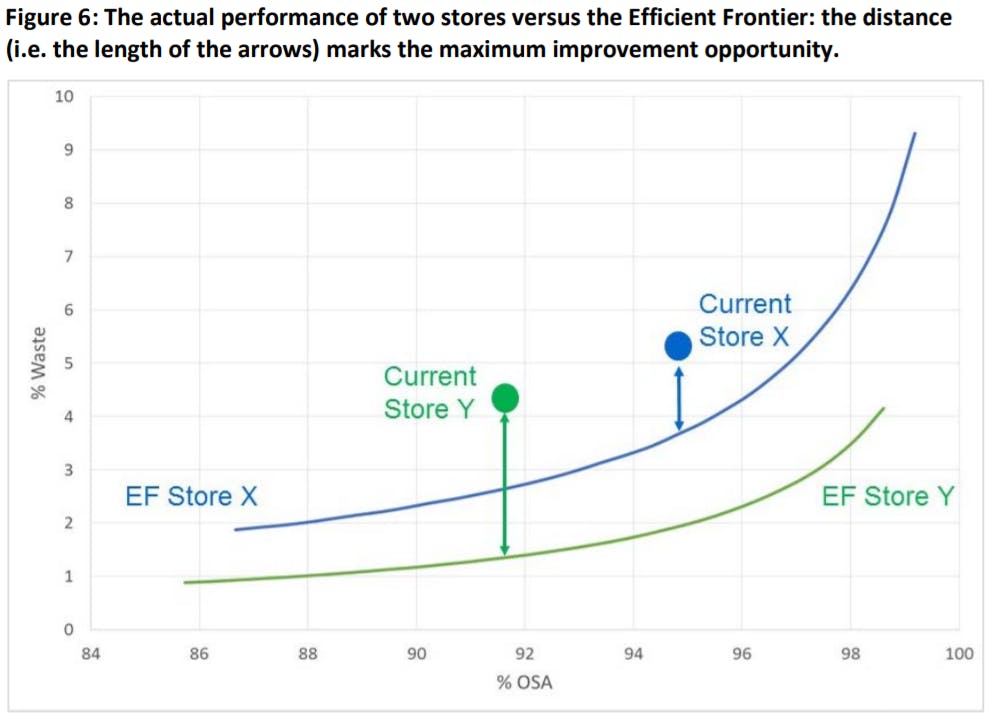
In Figure 6 the two Efficient Frontiers for two fictitious stores, store X and Y, are depicted. The actual performance of both stores are also added in the Figure. They are represented by the bold dots with the text “Current store X”. From these graphs it becomes very clear how close the stores are to their Efficient Frontier. The distance to their Efficient Frontier indicates their maximum improvement potential. In Figure 6 this maximum improvement potential is indicated with the two arrows. In this case, while the actual waste percentage for store X is larger than for store Y, the maximum improvement potential for store Y is larger than for store X. A potential explanation could be that since store Y has very large average daily demand per item-store combination they could have achieved a very low waste percentage. If the headquarters do not fully recognise this potential (i.e.; by not having explicit formulas to calculate the expected waste for any specific store), they may have set the budget for waste for store Y too high. Thus, they may have taken away the incentive for the person responsible for waste in store Y to further reduce waste, while a substantial further reduction is possible without reducing the OSA.
The distance from the Efficient Frontier is defined as:
%DistanceFromBenchmark = 100%*(WasteActual – WasteEstimated)/WasteActual
The method described above is applied for each of the 27 participating supermarkets to determine the distance between their actual performance and their Efficient Frontier. To determine the Efficient Frontiers for the 27 supermarkets in this analysis a target OSA is used. This OSA target has been determined based on discussions with the retailers. The results are summarised in Figure 7. On the horizontal axis the median Fresh Case Cover per store (taking into account all items in the store) is used. On the vertical axis the percentage distance from the Efficient Frontier is depicted, indicating the maximum improvement potential per store which is due to (amongst other things) store replenishment and execution.
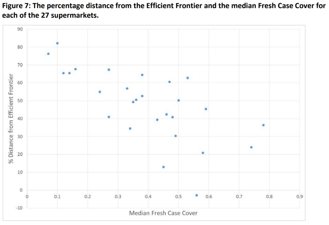
Two major observations follow from these results. First, the results show that the maximum improvement potential due to imperfect store replenishment and execution is very large: on average the maximum waste reduction per store by improving store replenishment and execution is equal to 48%. Second, the differences between stores are very large. While the five stores with the highest improvement potential have approximately 72% more waste compared with the benchmark, the five stores with the lowest improvement potential only have 17% more waste compared with the benchmark. The stores with the highest improvement potential are the stores with the lowest FCC, while the stores with the lowest improvement potential are the stores with the highest FCC. Another observation from Figure 7 is that stores with similar medium FCC values (in the range 0.3 to 0.5) vary widely in improvement potential. This shows that the level of demand (store dependent) and the supply chain parameters case pack size and store shelf life (retail chain dependent) are not sufficient to explain the percentage waste, since we see such a variation in the distance to the efficient frontier. Additional analyses may help to reveal the causes for this.
It is important to note that the percentage distance from the Efficient Frontier gives us the maximum improvement potential per store. According to the participating retailers part of the actual waste which is registered is not due to expiration, but for example due to goods being damaged by consumers when selecting the consumer units they prefer most or goods which accidentally get damaged during storage in the DC or during transportation. Although at the retail chain level this part of the waste is relatively small, it may still be relatively substantial for stores having very high sales: these stores typically have a low waste percentage and hence for these stores a 0.5% or 1% waste (as a percentage of sales) due to non-expiration issues is still relatively high. With almost no waste due to expiration, the loss due to damage becomes a relatively important factor. The stores having the highest %Distance from the Efficient Frontier are also the stores with the highest sales. Hence the improvement potential due to improved store replenishment and execution is likely to be somewhat smaller than indicated by the %Distance from the Efficient Frontier in Figure 7.
Recommendations
In this Section recommendations will be given to retailers and their suppliers, which will help to improve their performance on waste and/or sales. These recommendations are based on the results presented in the previous Section.
Recommendation 1:
Find the optimal mix between OSA and %Waste by selecting the sweet spot on the Efficient Frontier
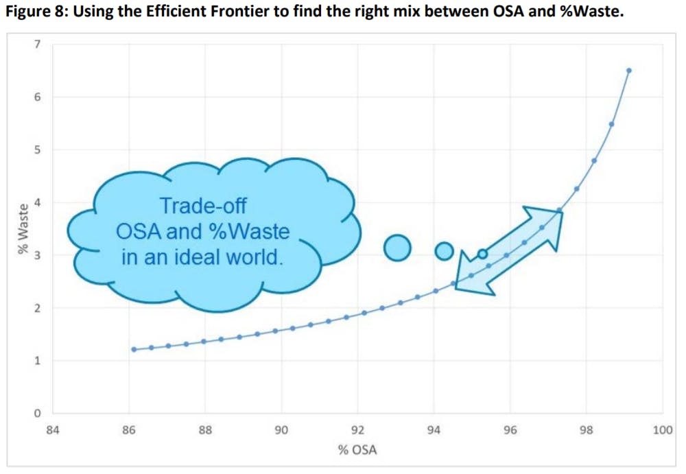
Determining the On Shelf Availability (OSA) target is a strategic decision for retailers which should be aligned with their marketing strategy. Retailers with a strategy focussed on high customer service typically aim for a very high OSA target. In this project OSA is defined as the percentage of customers demand satisfied from the shelf immediately. While retailers with a focus on high customer service typically aim for an OSA target equal to at least 98% for dry groceries, for perishables they typically aim for a lower OSA since the OSA target has a direct impact on the amount of waste. According to the Efficient Frontier in Figure 3 (and in Figure 8 below) a 98% OSA would imply 4.5% waste in an ideal world (and hence even more in the real world). Such a high level is not profitable for most retailers so they typically aim for a lower OSA for perishable items.
To find the optimal mix between OSA and %Waste, again the Efficient Frontier can be used. The Efficient Frontier shows the retailer how the %Waste changes if the retailer changes the OSA target. This trade-off is visualised in Figure 8. Essentially retailers will in this way select the sweet spot on the Efficient Frontier.
As will be shown in Tables 4 and 5 later on, it may be beneficial for a retailer to make separate tradeoffs for different parts of their assortments, for example for fast movers and slow movers or for items with a small shelf life and items with a medium to high shelf life. Then they will create separate Efficient Frontiers for these different parts of their assortment.
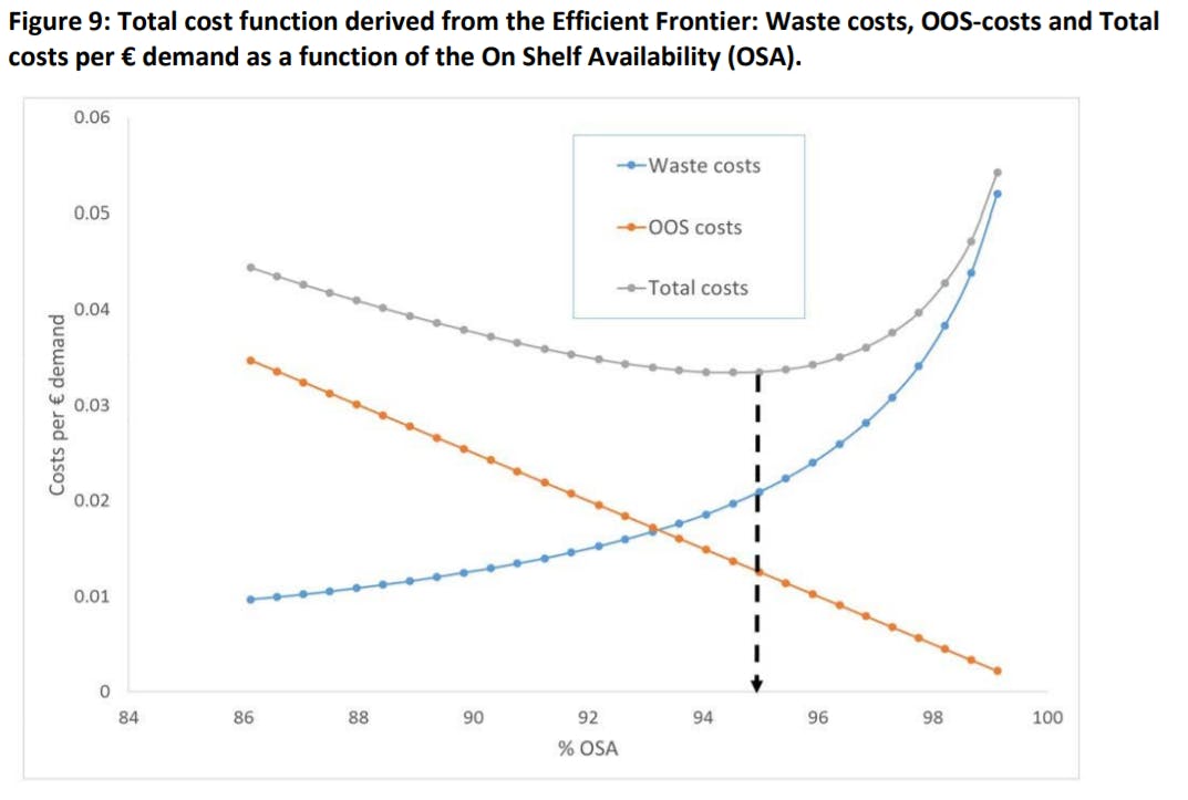
An alternative way for retailers to set the OSA target is to translate the Efficient Frontier into a total cost function. Depending on the costs of waste and the costs of out-of-stock retailers can make a trade-off and determine the optimal OSA target. The translation from the Efficient Frontier to the total cost function is especially easy if all items in the dataset underlying the Efficient Frontier are similar in sales price, margin and out-of-stock costs per consumer unit. In that case the Efficient Frontier can be translated directly into Figure 9, which shows how the total relevant costs depend on the target OSA. The total relevant costs are equal to the waste costs plus the out of stock costs. For this translation from the Efficient Frontier to Figure 9 the following fictitious margin, cost and substitution data are assumed: the profit margin (=sales price – purchasing price – supply chain costs) is equal to 20% of the sales price, the cost of waste is equal to (the sales price minus the profit margin) which in this case is 80% of the sales price, the percentage of customers willing to substitute to another item available in this store if their preferred item is out-of-stock = 75% and the lost sales costs per consumer unit (in case an item is out-of-stock and the customer is not willing to substitute) is equal to the sales price. Note that the lost sales costs are likely to be higher than the profit margin, since customers who do not want to substitute when confronted with an out-of-stock may decide to buy the item in another store and then they are likely to buy other items as well in the competitor’s store.
With these fictitious data the Waste Costs, the OOS-costs and the sum of both, i.e. the Total costs per € demand can be calculated from the %Waste and the %Lost Sales (which are reported in the Efficient Frontier, i.e. Figure 3 and Figure 8). Figure 9 shows how the costs depend on the OSA target. From this graph it can be easily seen that the optimal OSA target will be close to 95%. The graph also shows that in this case the total costs are rather flat around the optimum value, suggesting that topmanagement may decide to deviate from the optimal OSA target without large implications for the total resulting costs if they feel that other (e.g. qualitative or strategic) considerations are not taken into account in this simple cost model. By changing the parameters in the simple model (e.g. the lost sales costs) they can also do a sensitivity analysis to see how a change in parameters effects the results.
The graphs in Figure 9 confirm that for perishables waste costs are important: near the optimal OSA the waste costs are even larger than the OOS-costs. It also shows that a zero waste policy is far from optimal. Then the total costs would be much higher than in the optimal scenario and the OSA would be unacceptably low for consumers. So, while aiming for zero waste at the retailer level is not a realistic option, retailers can still influence the amount of waste by finding the right mix between waste and OSA.
The cost analysis above is made using the Efficient Frontier for all 17,093 item-store combinations. In practice it is suggested to do this analysis per retail chain at the product (sub) category level using separate Efficient Frontiers and/or separate cost functions for product categories which are very different in e.g. shelf life, average daily demand, case pack size or margin, cost and substitution parameters. The result from this differentiation will be that different product categories may need different OSA targets.
Recommendation 2:
Develop strategies to shift the Efficient Frontier
Apart from finding the right mix between OSA and %Waste, there are many other improvement opportunities for retailers. Given the fact that available time from employees and project team members to work on waste reduction as well as available budgets are often limited, top-management may want to prioritise the improvement opportunities. Below five improvement projects will be considered and it will be shown for each of these projects how the benchmarking tool can be used to quantify the effects on OSA and %Waste. This can assist top-management in prioritising the improvement projects. Among the five projects one project deals with reducing the case pack size and one project deals with increasing the shelf life for any item. At first sight these variables seem fixed, but actually in many situations they are the result of some decision making in the past and this decision did not necessarily include the effects of waste, for example because buyers were focussed on lowest purchasing prices only. Another potential reason for this is that up till recently no simple tool was available to quantify the effects of these decisions on waste. With the “Sell More, Waste Less”-tool being available to any retailer now, it is now possible to make a more informed decision taking effects on waste and OSA into account.
The following five improvement projects will be evaluated:
- Increase shelf life by one day
- Unpack all items in DC (case pack size store is 1) and ship smaller quantities to stores
- Reduce service levels: reduce the OSA by 2% for all item-store combinations
- Differentiate service levels: reduce OSA by 3% only for slow movers (defined here as the set of item-store combinations with the lowest average daily sales which make up 80% of the assortment) while increasing the OSA for the fast movers 5. Delist 10% from the assortment (ultra-slow movers, which results in 0.6% less sales if all customers decide not to substitute)
By increasing the shelf life or decreasing the case pack size (with projects 1 or 2), essentially the Fresh Case Cover is structurally decreased.
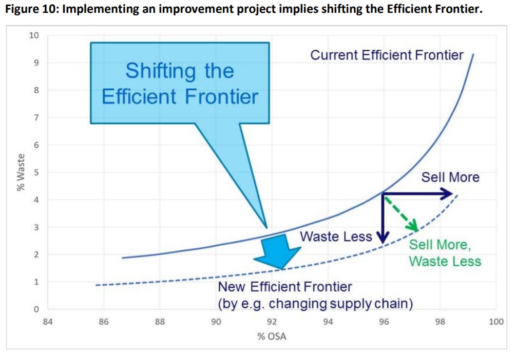
Implementing any of the above five improvement projects basically implies shifting the Efficient Frontier (see Figure 10). In Figure 10 the solid line represents the current Efficient Frontier and the dotted line represents the new Efficient Frontier (after implementation of the improvement project). Thanks to the improvement, the same OSA can be achieved with less waste (indicated by the arrow directing to “Waste Less” in Figure 10). In this case the waste can be reduced with approximately 45%: from 4.2% waste to 2.3% waste. Depending on its strategy and its current performance in comparison with competitors a retailer may also decide to use the improvement project to increase the OSA, while keeping the %Waste constant (indicated by the arrow directing to “Sell More”). In this case the OSA can be increased from 96% to 98.5%. Finally, the arrow directing to “Sell More, Waste Less” in Figure 10 shows that the retailer can select any point on the new Efficient Frontier in between these two extreme points and hence is able to Sell More AND Waste Less.
For the five improvement projects mentioned, the impact on the Key Performance Indicators can be calculated using the benchmarking tool. The results will be reported for the two extreme strategies the retailer can choose: either to use the benefits from the improvement projects to increase OSA as much as possible (while keeping waste constant) or to use the benefits to reduce waste as much as possible (while keeping OSA constant). Table 4 shows the effects on %Waste and OSA for each of the improvement projects if the objective is to Sell More, while Table 5 shows the effects on %Waste and OSA for each of the improvement projects if the objective is to Waste Less.
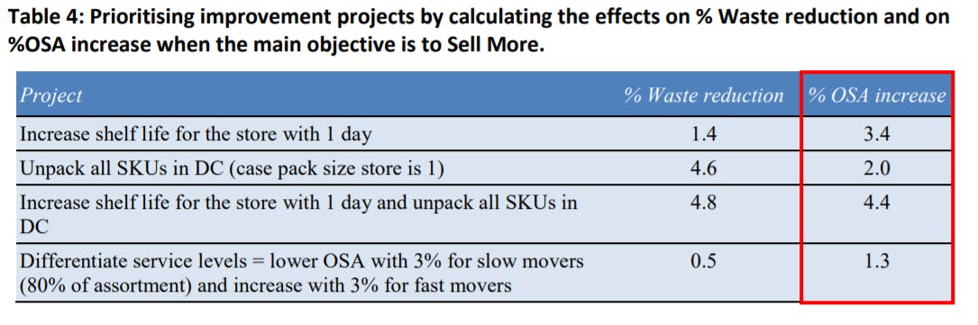
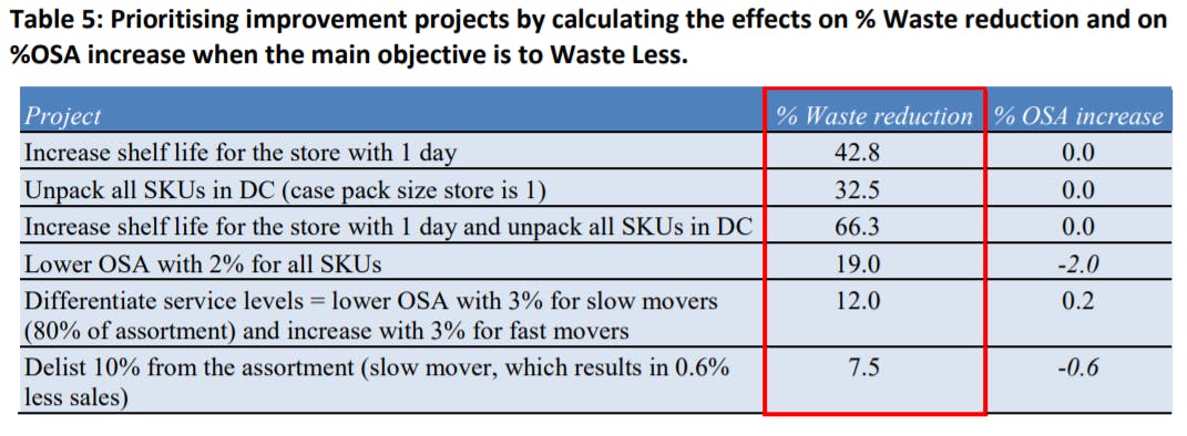
In the Sell More improvement projects, the main benefit comes from increasing the availability on the shelf, by having more time to sell the product (due to a longer shelf life), by increasing the potential delivery frequency (due to a smaller case pack size), or by fine-tuning the target inventory level. In the Waste Less improvement projects, we lower the Fresh Case Cover and thereby reduce the risk of waste, as was shown in Figure 5.
In both Tables it is assumed that each improvement project is applied for the items in the three product categories for all 27 stores. Making the calculations in this way shows that increasing the shelf life by just one day is the improvement project with the biggest potential, independent on whether the management objective is to Sell More or to Waste Less.
The second best improvement project when applied to all products and all 3 retailers in the database is the unpacking at the DC, i.e. delivering in the most flexible way to the stores without any restriction on the minimal order quantity. Of course, when implementing this idea in practice, it should be focussed on the items with the highest Fresh Case Cover since then the waste reduction potential is largest. If it would be applied to all items, the number of order lines will become unnecessarily high leading to unnecessarily high fixed handling costs.
The third row in both tables shows the benefits when both the shelf life is reduced with one day and all items are unpacked in the DC. As expected, the benefits from these combined improvements is less than the sum of the benefits from the individual improvement projects.
The fourth row in Table 5 shows that a substantial reduction in waste (-19%) can be achieved by reducing the OSA by 2 percentage points. This we know from the model, and it will depend on the costs of waste and the willingness of customers to substitute in case of an out-of-stock and the view of the Marketing team as to whether this is a feasible solution.
A relatively simple solution however is to improve the performance by differentiating the service levels. If for example the OSA is reduced by 3 percentage points for the slow movers, while at the same time the OSA for fast movers is increased, the total weighted OSA for the total assortment actually increases by 1.3% if the objective is to Sell More. This is caused by the fact that the total sales of fast movers is much higher than the total sales of all slow movers and hence customers benefit more from an increase in OSA for the fast movers than from a decrease in the OSA for slow movers. Although this is not the improvement project with the highest benefit, it is relatively easy to implement and actually some retailers already have implemented this kind of differentiation especially for categories with (very) low shelf lives and high willingness to substitute, like the bread category. When implementing the idea of service differentiation, different criteria can be used to differentiate, e.g. based on profit margin, willingness to substitute, sales and shelf life (see e.g. Van Donselaar et al., 2006).
The last improvement project evaluated here is the delisting of ultra-slow movers. Due to their very low daily sales they typically have a high percentage of waste and as a result they often are classified as “bleeders”, implying they have a negative contribution to profit (Werre, 2015). If 10% of the assortment with the lowest average daily sales would be delisted, the total waste would be reduced by 7.5% at the expense of an overall decrease of 0.6% of OSA if all customers who buy these products would not be willing to substitute. Clearly this is not the case: for many of these items only part of the customers are willing to substitute. This does not imply that all these bleeders should be eliminated. If products have just been introduced (say less than a few weeks), the daily sales may still grow over time as consumers learn to appreciate the new product. However, as shown in (Fisher and Raman, 1996) and (Fisher et al., 2001) in a different retail context (fashion retail), early sales information from the first weeks after a product introduction are a very strong indicator for the longer term sales potential and hence a critical review of keeping items in the assortment or not can often be done quite soon after the product introduction. The delisting of products also offers an opportunity to introduce other new products with a higher sales potential and lower waste or an opportunity to gradually reduce the assortment to enable more cost-efficient operations while keeping a close eye on how customers react to a slightly reduced assortment. When interviewing both large manufacturers of perishable products as well as supermarket owners and managers of fresh departments, they often expressed the opinion that in the last decade the assortments have grown substantially and they expressed concern that assortments are now too large. As one supermarket owner expressed it: “We sell more than 12 different types of pre-packed salad mix which are all very similar. I do not mind if at the end of the day only 8 of the 12 types of these salad mixes are available on the shelves, otherwise there will be too much waste”.
When interpreting the results presented in Table 4 and Table 5, it is important to note that for most improvement projects some other costs (e.g. investment, implementation or change costs) or qualitative arguments have to be included in the final decision process to determine which improvement projects are most attractive per retailer. For example, handling costs are also an important cost component in food retail. For dry groceries handling costs in both the stores and DC represent 66% of the total supply chain costs (Van Zelst et al. 2007). As mentioned, reduction of case pack sizes will increase the number of order lines ordered by the supermarkets. More order lines imply higher handling costs both in the supermarket (searching for the product on the shelf and taking out older products to put the fresh items in the back of the shelf) and the DC (more order lines per trip in the DC implies extra searching and picking time). Hence when retailers want to evaluate the total impact of reducing case pack sizes, not only OSA and %Waste are relevant KPI’s, but also the number of order lines. For this purpose, the “Sell More, Waste Less” tool which is made available to retailers and their suppliers reports multiple KPI’s, including OSA, %Waste, Number of order lines and Freshness to consumer.
Recommendation 2a: Use your own data to quantify the improvement potential
When the calculations above are redone for each of the three retailers separately, it turns out that actually the improvement project with the biggest potential to reduce waste may differ per retailer. Probably this is due to the focus which have been given to different aspects in the past: some retailers may have worked already very intensively with suppliers, the DC and the stores to increase the shelf life and reduce lead times and inventories in the supply chain while others may have invested already in differentiating and redesigning warehouse operations to allow for efficient handling of small case pack sizes for fresh items with low shelf lives and other retailers may have invested recently in advanced automated forecasting and replenishment systems. The fact that different retailers may have different improvement projects with the highest potential shows it is worthwhile for any retailer who wants to identify the best potential improvement project(s) to make these calculations for their specific situation using company specific data.
If for example a company wants to calculate the waste reduction potential when increasing the shelf lives for a subset of their items, it starts with providing the following input data in an empty worksheet of the “Sell More, Waste Less” tool: per item-store combination the item number, the store identification (and optional the item description and the store name for easy reference), the average daily sales, the case pack size, the shelf life and the target %OSA. This input can look like the following snapshot:
This input is then used to calculate the standard deviation of the daily demand (using the simple formula in Section 2.2), the reorder level, the resulting %OSA (which may be higher than the target %OSA since reorder levels can only have discrete numbers) and the resulting %Waste. The calculation of these last three fields are done with the standard functions provided in the “Sell More, Waste Less” tool. These standard functions and their required input are described in the user manual which is attached in Appendix 1. The calculation of the resulting %Waste is done twice: for the current shelf life and for the shelf life plus one day. The reorder level and the resulting %OSA are independent of the shelf life when the smart replenishment logic is used as assumed in the “Sell More, Waste Less” tool, so these two numbers only have to be calculated once per item-store combination. The calculations result then in a Table which looks like the following snapshot:
By using the waste percentages in the last two columns the retailer can determine how much waste can be reduced if the shelf life is increased with one day for this subset of items.
Recommendation 2b: When increasing shelf life by one day, focus on items with shelf lives up to 8 days
While total waste is reduced by 42.8% if the shelf lives of all item-store combinations are increased by one day (see Table 5), total waste is reduced by 40.1% if only the item store combinations with a shelf life of between 3 and 8 days are increased by one day. Note that items with one or two days shelf life (e.g. bread) are not included in the database. The item-store combinations with a shelf life of between 3 and 8 days make up 50% of the all item-store combinations in the database, but are responsible for 93.8% (=40.1/42.8) of the potential to reduce waste by increasing shelf life by one day.
The explanation for this is twofold: the item-store combination with shelf life between 3 and 8 days are relatively fast moving (these 50% of the item-store combinations create 84% of total consumer units sold) and an increase in shelf life by one day gives a higher percentage waste reduction for lower shelf lives. Increasing for example the shelf life when the current shelf life is 3 or 4 days typically results in more than 50% waste reduction, while increasing the shelf life when the current shelf life is 28 or 29 days, typically results in only a 10% waste reduction. For these two reasons, it is recommended for companies aiming to increase their shelf lives, to focus mainly on items having a shelf life up to 8 days.
Recommendation 3:
Determine how Fresh Case Cover is driving your waste.
Every retailer can replicate Figure 5 for his own organisation. The only data needed are for every item-store combination: the case pack size, the shelf life, the average daily sales and the percentage actual waste. With these data, the FCC can be calculated in Excel using the formula 𝐹𝐹𝐹𝐹𝐹𝐹 = 𝑄𝑄/(𝑚𝑚. 𝜇𝜇) (see the snapshot below).
Next, the Table should be sorted for the FCC values and finally for every class of FCC values the weighted average %waste should be calculated (according to the logic described in Section 3.2). With these numbers a graph similar to Figure 5 can be created. The retailer can thus verify whether the simple linear relationship between %Actual Waste and FCC, which is visible in Figure 5, also holds for his/her company. This graph is an extremely easy way to communicate to all employees in the retail organisation and its suppliers how three key variables (the case pack size, the shelf life, the average daily sales) determine to a large extent the amount of waste in the company. Moreover, category managers, supply chain managers, buyers and suppliers can easily identify which of their items have a high FCC and hence start a discussion whether it is worthwhile to reduce waste by reducing the FCC for the items having a high FCC value. The graph will give them a first indication how much waste can be reduced if they lower the FCC by increasing the shelf life, reducing the case pack size or increasing the average daily demand. This is only a first indication, which works well when applied to a very large group of item-store combinations. For a more accurate estimate of the waste reduction potential for individual items or a small set of item-store combinations, it is recommended to use the simple “Sell More, Waste Less” tool. Compared to the FCC, this tool also takes into account for example differences in target OSA levels when estimating the expected waste percentage. Although this tool is based on the ideal world, the difference between the real world and the actual world is relatively small when applied to situations with a high FCC.
Recommendation 4:
Benchmark stores and analyse their behaviour
With the methodology presented in Section 3.3 retailers are able to identify which stores and which fresh departments have the biggest gap between the actual performance and the benchmark. The output of this gap-analysis can act as a starting point for a meeting with managers from best-in-class stores and less-in-class stores in which best practices are shared. For example, imagine a retailer having 300 stores who wants to benchmark the departments selling the ready-made meals, each carrying 80 different items or a subset of it (depending on the total sales of the store). For every itemstore combination in this product category the retailer can collect the average daily sales, the case pack size, the shelf life and the target %OSA. With these input data the retailer can determine the reorder level, the resulting %OSA and the resulting %Waste for each item-store combination using the standard functions in the “Sell More, Waste Less” tool (see Appendix 1 for the user manual of this tool and the explanation of these standard functions). When multiplying this resulting %Waste with the average daily sales the retailer gets for each item-store combination the expected waste expressed in consumer units per day in the ideal world (the benchmark). By summing these waste numbers over all items for each store separately the retailer can determine for every store the relative difference between the waste according to the benchmark and the actual waste reported by that store. This gives the retailer the “%Distance from Efficient Frontier” per store, which indicates which stores have the highest (or lowest) improvement potential from store replenishment and execution.
In addition, analysing in further detail a small sample of item-store combinations with the largest and the smallest gaps between the actual performance and the benchmark at item-store combination level, has proven to be a very efficient and effective way to identify the reasons why fresh departments outperform or underperform. When making a time-phased plot of the sales, supply and waste for those item-store combinations it became evident that in some cases the fresh managers structurally deviated from the advice of the automated store ordering system. Some fresh managers wasted much more than suggested by the benchmark. For example, a fresh manager structurally discarded fresh herbs only a few days after he received them and then ordered new supply, while according to the shelf life these products could be sold for many more days. In other cases this kind of outlier-gap-analysis showed that some stores were creative in finding ways to do even better than the performance which could be reached in the ideal world. One way to achieve this was by not ordering an expensive slow moving item for 1 or 2 weeks every time when one or a few consumer items of this product were wasted (so the manager of this fresh department frequently decided to temporarily delist the item). Another local solution, only possible for products without an explicit sell by date set by the supplier, was using dynamic expiration dates based on the actual quality level of the products entering the store. This creates the opportunity to sell items for a longer period than the more conservative period we used in the benchmark. In a discussion with the regional store operations manager (responsible for advising the stores) it can be evaluated whether this better performance is due to a smart solution from the local fresh manager which can be shared with her/his colleagues or whether this solution is not in line with other strategic objectives of the retail company and should be discouraged. This kind of performance analysis can also be the starting point of a review of the current store replenishment system or the development of a new replenishment system. For example, taking into account an estimate for tomorrow’s waste when deciding on the replenishment quantity or using an aggregate inventory target for a group of products with high substitution willingness (i.e. first determining the desired total number of products (e.g. in kilograms) for the entire product category in a store and then breaking it down to the item-store combinations) are ways to improve the performance of the fresh departments.
Recommendation 5:
Use the 65 point checklist to identify new ideas to reduce waste
Thus far, the analyses in this report have focused strongly on improvement suggestions related to changing four key drivers of waste: the target OSA level, the shelf life, the case pack size and the average daily demand. Yet there are many other improvement opportunities. For example related to the replenishment logic, the way products are displayed in the stores (some managers adhere to the principle “Pile them high, Let them fly”), the way products are stored (temperature and light conditions), training people and giving people the right incentives. In Appendix 2 a checklist is provided with 65 suggestions which may help to reduce waste and/or increase sales in the fresh departments. This checklist is based on interviews with many retailers and a literature review.
Limitations and future research
In Section 2.2 two limitations and two assumptions made throughout the research project have been discussed. The two limitations are the fact that the weekly pattern is not taken into account since sales are assumed to be constant throughout the week and the fact that the effect of price discounts (when items near their expiration date) on sales rate are not included. The two assumptions dealt with the replenishment logic and the customer withdrawal behaviour. It is assumed retailers use a smart replenishment logic which takes the expected amount of waste into account when a new replenishment order is generated and it is assumed that the percentage of customers buying the freshest items on the shelf has limited impact on the amount of waste as long as this percentage is not very high.
For the impact of the weekly pattern and the customer withdrawal policy some first results are available, suggesting the impact is limited. For the impact of discounts when the item nears their expiration date, retailers have done empirical tests, but few of these test results are published. Further research may be devoted to study these issues in more detail and in a more rigorous way.
The smart replenishment logic may be applied by fresh department managers when they create the replenishment orders manually and when they keep track of the oldest items on the shelves. Automated Store Ordering systems typically do not include this replenishment logic since the information system does not contain detailed information on the age-build-up of the inventories on the shelf. For retailers having a lead time and a review period equal to one day and which discount the fresh items the night before the expiration date, the EWA logic can be used without any additional information on the age-build-up of the inventories. A topic for future research is to develop for the other retailers a new replenishment logic, which is not based on the detailed age-build-up of the inventories, but which assumes that the expiration date is known for each batch which enters the store.
The assumption that the lead time and review period is one day is only needed when using the “Sell More, Waste Less” tool in its current form. This tool can easily be extended to situations with lead time and/or review periods equal to two days, thus covering most of the situations retailers will encounter. Suppliers however may be dealing with longer lead times and review periods. Future research can evaluate whether it is sufficient for suppliers to normalise their time-based data (e.g. using weeks rather than days) and still use the existing theory or whether new approximations for waste have to be developed for situations with long lead time and/or review periods.
Other topics for future research include:
- An investigation on how to further support the decision makers in the fresh supply chain with information on waste and OSA. For example how to support a category manager who is confronted with a large number of developments, issues and information when (s)he is making a new planogram; should information on waste and OSA be made visible or should the information be included in an algorithm which provides a preliminary planogram which can then be improved by the category manager? If included in an algorithm, how should the algorithm use this information on waste and OSA?
- A study on how to organise for a more Efficient Frontier. For example: What are the (dis)advantages of creating the position of a Chief Fresh Officer and/or setting up a Fresh project team? Which incentives to create throughout the supply chain and at different organisational departments to ensure full cooperation of all people involved in the change process?
- An extension of the checklist on improvement suggestions to reduce waste and/or increase sales, provided in Appendix 2. For example by analysing which interventions are relatively simple to implement, which ones are most valuable in terms of reaching the objectives and which ones require the smallest investment. Each of the improvement opportunities suggested there can also be worked out in more detail, thus making it easier for the retailers to implement these suggestions
- An empirical analysis of different causes for the part of the food waste in stores which is independent of the expiration date, clarifying both the magnitude of this part of the food waste in retail and which factors are driving this part of the food waste
- A documentation of case studies from retailers working successfully on waste reduction and sales increase in their fresh departments
References
Broekmeulen, R.A.C.M., van Donselaar, K.H., 2009. A heuristic to manage perishable inventory with batch ordering, positive lead-times and time-varying demand. Computers & Operations Research 36(11), 3013–3018.
Buzby, J. C., Wells, H.F., Hyman, J., 2014. The Estimated Amount, Value, and Calories of Postharvest Food Losses at the Retail and Consumer Levels in the United States, USDA Economic Research Service, Economic Information Bulletin 121.
Buzby, J. C., Bentley, J.T., Padera, B., Ammon, C., Campuzano, J., 2015, Estimated Fresh Produce Shrink and Food Loss in U.S. Supermarkets. Agriculture, 5(3), 626-648. Published online August 4, 2015. http://www.mdpi.com/2077-0472/5/3/626.
Eriksson, M., Strid, I., Hansson, P., 2014, Waste of organic and conventional meat and dairy products—A case study from Swedish retail, Resources, Conservation and Recycling 83, 44– 52.
Fernie, J., Sparks, L., 2009, Tesco’s supply chain management. In: J. Fernie and L. Sparks, Logistics and retail management (p.143-169). London: Kogan Page.
Fisher, M., Raman, A., 1996, Reducing the cost of demand uncertainty through accurate response to early sales, Operations Research 44(1), 87-99.
Fisher, M.; Rajaram, K. and A. Raman, 2001, Optimizing Inventory Replenishment of Retail Fashion Products, Manufacturing & Service Operations Management 3(3), 230-241.
Gustavsson, J., Cederberg, C., Sonesson, U., 2011. Global food losses and food waste. Gothenburg, Sweden, http://www.fao.org/docrep/014/mb060e/mb060e.pdf.
Lebersorger, S., Schneider, F., 2014, Food loss rates at the food retail, influencing factors and reasons as a basis for waste prevention measures, Waste Management 34, 1911–1919.
Lütke Entrup, M., 2006, Advanced planning in fresh food industries: integrating shelf life into production planning. Springer.
Oliver Wyman, 2014, Reducing food waste; how can retailers help? http://www.oliverwyman.com/content/dam/oliverwyman/global/en/2014/jul/OW_Reducing_Food_Waste.pdf
Silver, E.A., Pyke, D.F., Peterson, R.,1998, Inventory Management and Production Planning and Scheduling (3th ed.). Chichester:
Wiley. Tromp, S.O., Rijgersberg, H., Pereirada Silva, F. Bartels, P. (2012) Retail benefits of dynamic expiry dates: Simulating opportunity losses due to product loss, discount policy and out-of-stock, International Journal of Production Economics 139, 14–21.
Van der Vlist, P., R.A.C.M. Broekmeulen, 2006, Retail Consolidation in Synchronized Supply Chains. Zeitschrift für Betriebswissenschaft, H2, 1-12.
Van Donselaar, K.H., van Woensel, T, Broekmeulen, R.A.C.M., Fransoo, J., 2006, Inventory control of perishables in supermarkets. International Journal of Production Economics 104, 462–472.
Van Donselaar K.H., Gaur V., van Woensel T., Broekmeulen R.A.C.M., Fransoo J.C., 2010, Ordering behavior in retail stores and implications for automatic replenishment. Management Science 56(5), 766-784.
Van Donselaar, K.H., Broekmeulen, R.A.C.M., 2012, Approximations for the relative outdating of perishable products by combining stochastic modeling, simulation and regression modeling. International Journal of Production Economics 140, 660–669.
Van Donselaar, K.H., Broekmeulen, R.A.C.M., 2013, Determination of safety stocks in a lost sales inventory system with periodic review, positive lead-time, lot-sizing and a target fill rate. International Journal of Production Economics 143(2), 440-448.
Van Woensel, T., van Donselaar, K., Broekmeulen, R., Fransoo, J., 2007, Consumer responses to shelf out-of-stocks of perishable products, International Journal of Physical Distribution & Logistics Management, 37(9), 704-718.
Van Zelst, S., van Donselaar, K., van Woensel, T., Broekmeulen, R. Fransoo, J., 2009, Logistics drivers for shelf stacking in grocery retail stores: Potential for efficiency improvement, International Journal of Production Economics 121, 620–632.
Werre, P, 2015, Waste reduction Albert Heijn, case study presented at the “Sell More, Waste Less” seminar in London, Oct 20, 2015, http://www.ecr-shrinkgroup.com/food_waste_workshop/albert_heijn_presentation_-_peter_werre.pdf
WRAP, 2011, Reducing Food Waste through Retail Supply Chain Collaboration, report by James Tupper and Peter Whitehead, http://www.wrap.org.uk/sites/files/wrap/WRAP_IGD_supply_chain_report.pdf
WRAP, 2015, “Sell More, Waste Less”, presentation by Sue Riley at the “Sell More, Waste Less” seminar in London, Oct 20, 2015. http://www.ecr-shrinkgroup.com/food_waste_workshop/wrap_overview_-_sue_riley.pdf
Appendices
A: User manual for the “Sell More, Waste Less” tool
Introduction
The “Sell More, Waste Less” tool is a Excel file with macros to calculate several Key Performance Indicators (KPI’s) for the inventory systems at retail stores, specific for fresh (perishable) items.
- On Shelf Availability (OSA): percentage of customer demand delivered from the shelf;
- Waste: total waste per period as a percentage of total demand in the same period. Both waste and demand are measured in consumer units (CU’s );
- Freshness to customer: the average number of remaining shelf life in days that the customer gets when buying the item;
- Number of order lines: the average number of order lines per day. If an item is ordered once every 20 days, this number is equal to 0.05;
- Probability non-empty shelf: the probability that the shelf for this item is not empty just before a new delivery is made for this item or another item in its category (i.e. when the store looks most empty);
The tool can handle many situations encountered in practice. This version for the ECR Community OSA & Shrinkage Group makes several restricting assumptions to achieve a better user experience, but most of these assumptions can be relaxed by using an advanced version of the tool.
- Lead time (between ordering and shelf stacking) is one day;
- Inventory review frequency (to determine replenishment orders) is once per day per category;
- Most shoppers buy oldest items first (FIFO)
- The store replenishment logic takes into account the number of items which expire tomorrow.
New users are advised to begin with reading the Section “Getting started” and to perform each of the five steps explained there using one of the two standard worksheets in the tool. Once users are familiar with the basics of the tool, they can start creating their own tailor made worksheets using the standard functions available in the “Sell More, Waste Less” tool. In the last Section of this manual it is explained how to do this.
Copyright notice and disclaimer
The “Sell More, Waste Less” tool has copyright, which means that all rights are held by the authors Broekmeulen & Van Donselaar. The tool may be used by the companies which are member of the ECR Community OSA & Shrinkage Group. While the authors made every effort to ensure that the tool is error-free, errors do occur. We ask that you notify us immediately of any errors that you discover in our tool. We will make every effort to correct them.
Getting started
Step 1: Open the Excel file that contains the tool
The tool is a macro-enabled Excel file (XLSM) and requires to be trusted by the operating system. When opening the Excel file, please enable the macro content, otherwise the added functionality is not available. For more information about enabling macros, see the website of Microsoft Office.
Step 2: Choose a worksheet, depending on the evaluation scenario
The parameters that determine the expected OSA and waste can be evaluated in two different scenarios. For each scenario a different worksheet is available:
- Efficient Frontier: in this scenario, a minimal target level for OSA can be set, based on the corresponding waste level according to the efficient frontier for the given parameters. This is a good starting point for evaluation;
- Cost trade off: in this scenario, the costs related to waste, out-of-stocks and ordering are shown as a function of the % OSA for the given parameters. This is suitable for retailers who prefer to minimize the total relevant costs.
Step 3A: Setting the basic parameters
In both scenarios, three basic product parameters are needed for the calculations (see top left corner of the worksheet, cells C4, C5 and C6):
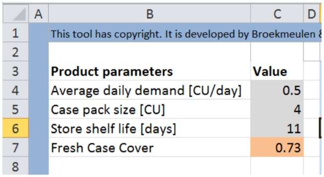
- Average daily demand [CU/day]: average demand per week in consumer units (CU) divided by 7 (to get demand per day);
- Case pack size [CU]: replenishment orders are in a multiple of this number;
- Store shelf life [days]: the average time in days between the arrival of an item in the store and its expiration date
If you need a reminder of the definition of these parameters, please click in the cell.
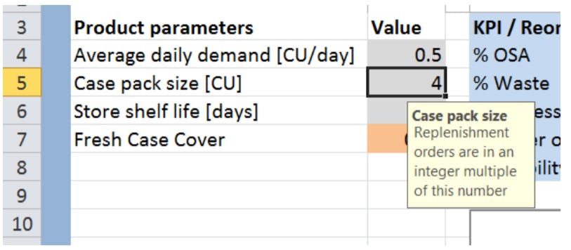
Step 3B: Setting the cost parameters (only for “Cost trade- off” scenario)
In the “Cost trade off” scenario, the tool needs four additional parameters for the calculations (see middle left side of the worksheet, cells C10, C11, C12 and C13):
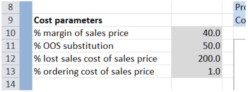
- % margin of sales price: gross margin as a percentage of the customer sales price;
- % OOS substitution: percentage of customers buying a substitute in the store if their preferred item is out of stock (OOS);
- % lost sales cost of sales price: the penalty cost per consumer unit, as a percentage of the sales price, if the customer faces a stock out and is unwilling to substitute;
- % ordering cost of sales price: the fixed ordering cost per order line as a percentage of the sales price per CU
Step 4: Read the output from the tool
The tool provides the user with graphs as well as detailed output for the KPI’s. In the graphs, the output is plotted as a function of the % OSA. The graph which shows how % Waste increases if % OSA increases is called the Efficient Frontier.
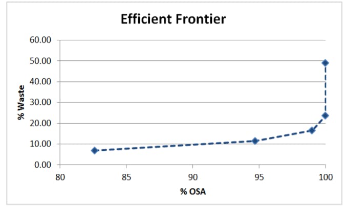
The detailed output is shown in the upper right corner.
The range F3:S3 shows different reorder levels. A reorder level is a target inventory level: if the inventory position for the item drops below this level, a new inventory replenishment order is created. The first value in this row starts with the reorder level for which the OSA is at least 80%. The subsequent rows show the resulting KPI’s for each reorder level.
In the “Efficient Frontier” scenario, the user selects the reorder level which meets her minimal target OSA. For example: if the minimal target OSA = 93%, the output of the tool above shows that the reorder level should be set equal to 2 consumer units. With this reorder level the resulting %OSA=94.7% and the resulting %Waste=11.4%. Note that the minimal target OSA levels cannot be reached exactly, due to the fact that reorder levels are always integer.
In the “Cost trade off” scenario, we have an additional output row: Cost per € demand. This is the total relevant costs per day divided by the potential turnover per day (i.e. when OSA=100%). The tool automatically highlights the minimal costs (in red, see below).
In addition, a graph is made which shows how the total relevant costs per € demand depend on the % OSA.
Step 5: What-if analyses
The user can do what-if analyses by changing the input parameters, such as case pack size and store shelf life. Consider the following example with an average daily demand of 0.5 CU/day, a case pack size of 4 CU and a store shelf life of 11 days. In the base scenario we have the following output:
When we increase the store shelf life with 1 day to 12 days, we get:
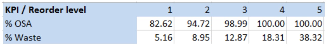
An alternative scenario is unpacking the case pack at the distribution centre; such that the store can order with a case pack size of 1 (store shelf life is back to 11 days).

Tips for calculating the right input parameters
For the functions, the input parameters must be within certain ranges to be valid, such as being nonnegative. The functions return error codes (starting from -9900) in case of invalid input values.
For determining the average daily demand, first determine the average weekly demand and then divide this by 7. When calculating the average weekly demand, make sure you exclude promotional weeks and weeks when the item was not on sale in the store. Although the tool makes no correction for a possible week pattern in sales, simulation studies revealed that the impact of this week pattern on the trade-off between % OSA and % Waste is limited.
When using cost or substitution parameters: please check whether these are different for different product categories or products.
Making tailor made worksheets using the standard functions
The experienced user can also make tailor made worksheets using the standard functions available in the “Sell More, Waste Less” tool. Three standard functions, which are often needed when making a tailor made worksheet, are:
- DoBr_TargetFillRateReorderLevel: calculates the lowest reorder level which will result in a service level (resulting %OSA) which is at least equal to a target service level (target % OSA);
- DoBr_FillRate: calculates the resulting service level (% OSA) for a given reorder level;
- DoBr_EZ: calculates the resulting % Waste for a given reorder level
Note that EZ in DoBr_EZ stands for the expectation of Z, with Z the variable used for the waste percentage in the scientific paper which is used to determine this number.
The easiest way to see which input parameters (function arguments) are needed for these three functions, is to click on fields F3, F4 or F5 in the worksheet “Efficient Frontier” or “Cost trade off” in the “Sell More, Waste Less” tool. Then the formula bar (visible at the top of the Excel file) will reveal the function and which input parameters are needed and in which sequence.
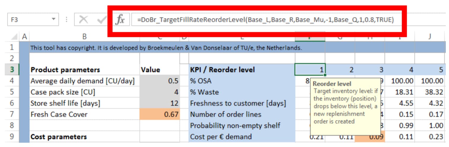
By clicking on the symbol 𝑓𝑓𝑥𝑥 just in front of this formula bar, a table will pop up, which provides the names of all input variables and which allows the user to enter specific values for these input variables.
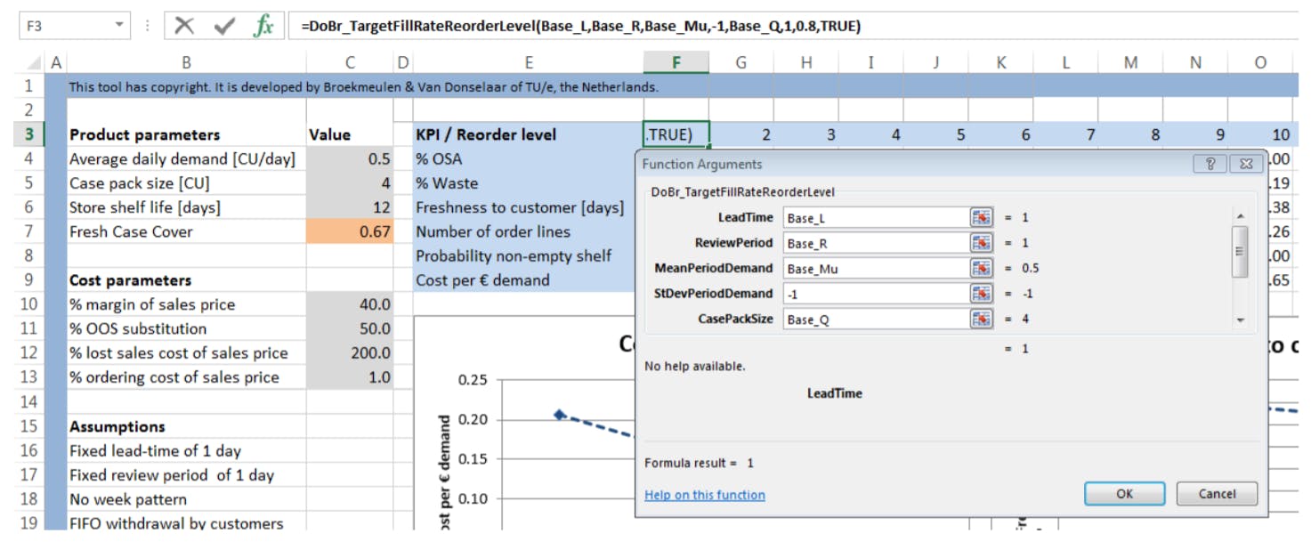
The input parameter for the average daily demand is called “MeanPeriodDemand”. To simplify the use of this tool, the user can simply fill in the value “-1” at “StDevPeriodDemand” if the user wants the tool to apply the function 𝜎𝜎 = 1.18 ∙ 𝜇𝜇0.77 to determine the standard deviation of daily demand. If the user does not want to use this formula, the user can specify in this field his/her own value for the standard deviation. For the input parameter MOQ, the value “1” should be entered. For the input parameter ‘TargetFillRate’ the target OSA should be entered (e.g. 0.95 should be entered if the OSA target is equal to 95%). For the input parameter Lost Sales, the value ‘TRUE’ should be entered. For the input parameter FIFO (in DoBr_EZ) the value “TRUE” should be entered. When entering the values for these input parameters, please remember to scroll down in the pop-up table to see all input parameters.
Each of these three standard functions can be used in any cell in any worksheet in the tool. By entering in any cell the text “=DoBr”, Excel will automatically show a list of all standard functions in the tool starting with these letters and the user can then simply select DoBr_TargetFillRateReorderLevel, DoBr_FillRate or DoBr_EZ. By double clicking on the desired standard function, the function will appear in the formula bar and the user can enter the values for the input parameters (either directly or (after clicking on the 𝑓𝑓𝑥𝑥 button) via the table with function arguments).
The tool contains many other standard functions and different options for input parameters to deal for example with LIFO instead of FIFO, with backordering situations (versus lost sales) and with reorder policies using minimum order quantities rather than base order quantities (like the case pack size). Experienced users interested in these options are invited to contact the authors for more details:
Email: r.a.c.m.broekmeulen@tue.nl or k.h.v.donselaar@tue.nl
Appendix
B. Checklist with improvement suggestions to reduce waste and/or increase sales for the fresh departments
There are several initiatives which have been taken or which can be taken by retailers and suppliers to reduce waste. In this Section we provide an overview of these initiatives. Retailers and their suppliers can use this overview as a checklist or as a source of inspiration to find new initiatives to reduce waste within their own organisation.
In Table A1 the improvement projects to reduce waste have been classified in two groups: projects with a focus on Supply Management and projects with a focus on Demand Management. It should be stressed that while the focus may be on either demand or supply management, waste reduction may involve multiple stake holders in the supply chain and people from different disciplines. Those type of improvement projects are only likely to be successful when waste reduction is considered a toppriority by the company’s senior-management.
Projects with a primary focus on supply management can be further classified into projects focusing on the store:
- Store operations management
- Shelf replenishment
- Inventory replenishment logic
- Case pack size
- Minimum stock
and projects focussing on the supply chain.
Projects with a primary focus on demand management can be further classified into projects focussing on:
- Level of demand
- Markdown strategy
- Customer withdrawal behaviour
- Demand uncertainty
- Demand dynamics
- Demand forecasting
- Promotion management
- Planograms/displays
- Assortment
While Table A1 can be seen as a check list containing many improvement opportunities to reduce waste, it is by no means intended to be an exhaustive list. All participants in waste reduction projects are encouraged to gather data on actual-performance versus benchmark-performance and then to start idea-generating sessions with both best-in-class and less-in-class performers to see how their experiences and ideas help to further extend the list of improvement opportunities or to adapt it to their specific situations.
Projects with a primary focus on SUPPLY management
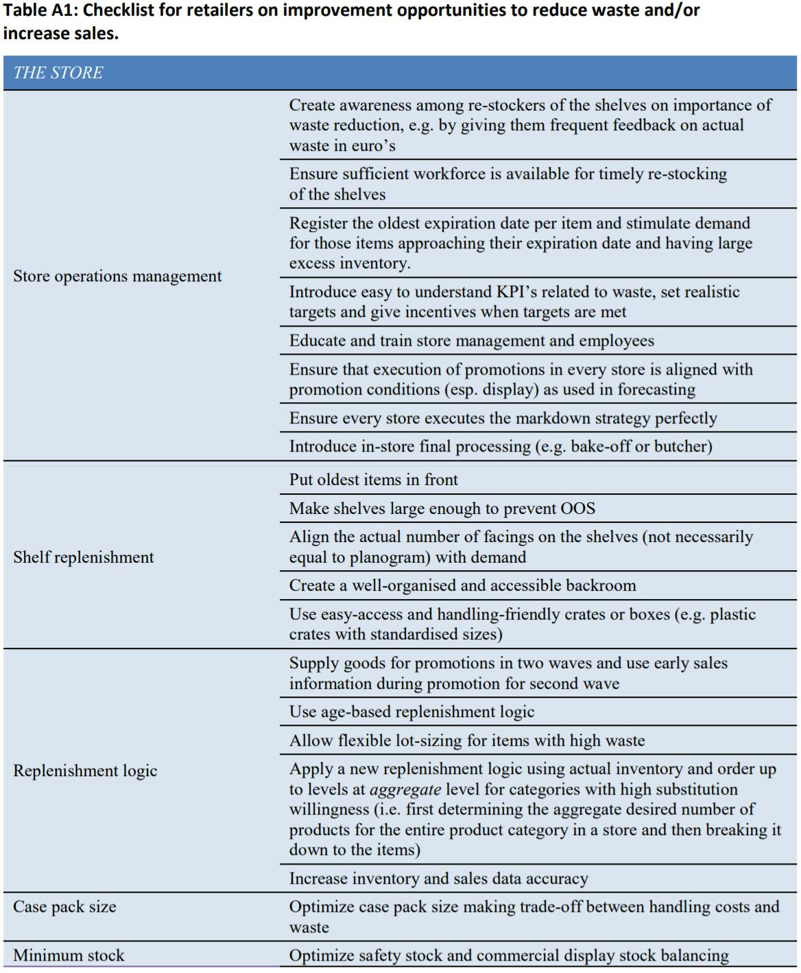
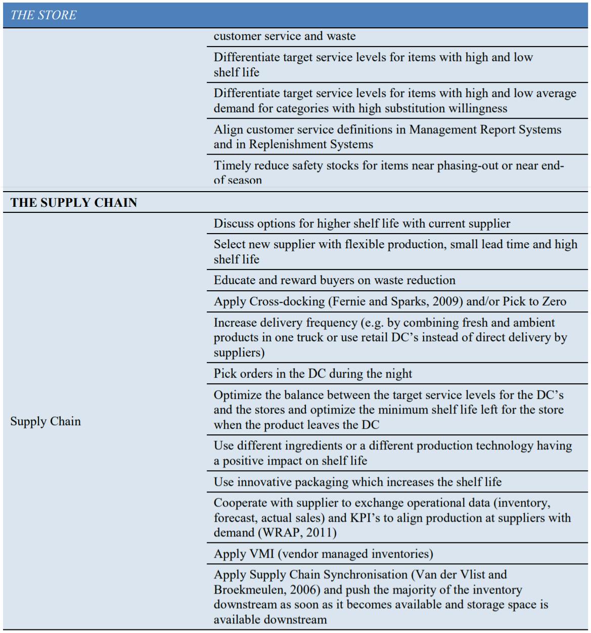
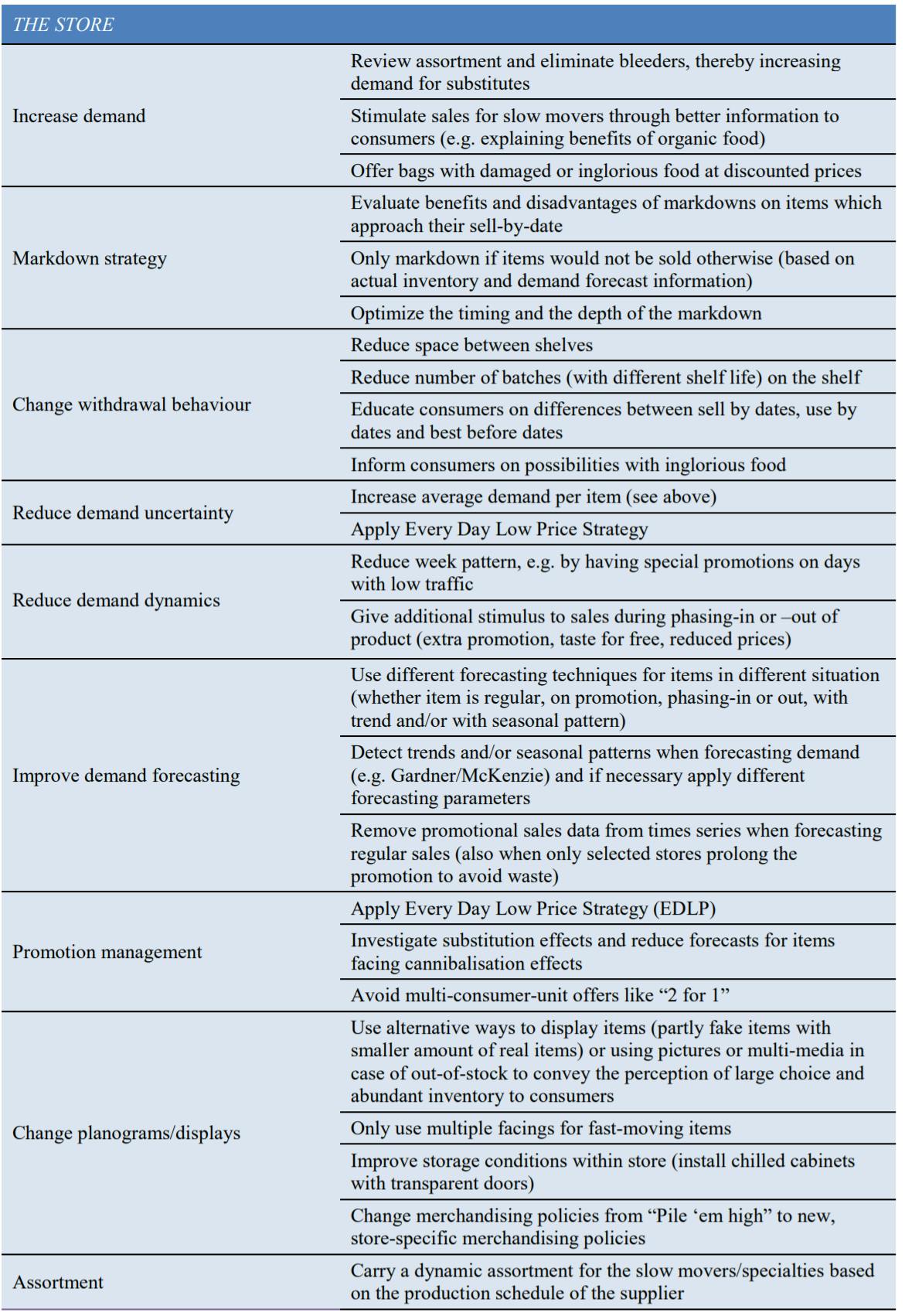


Main office
ECR Community a.s.b.l
Upcoming Meetings
Join Our Mailing List
Subscribe© 2023 ECR Retails Loss. All Rights Reserved|Privacy Policy