This report explores the impact of significant changes in the rate of inflation on the measurement of retail loss. The key finding is that it is not the rate of inflation itself, but the effects of inflation on consumers' behaviour and retailers' decisions that is responsible for the changes seen in the Key Performance Indicator, Retail Loss %. As a result, retailers are encouraged to explore other measures of loss that reflect changes in units rather than in prices, and to reflect that 'when a measure becomes a target, it ceases to be a good measure' (Goodhart's Law).

Until very recently, we have lived through a long period of relatively low levels of inflation. However, as economies have emerged from the effects of the global COVID Pandemic, rates of inflation have risen to levels not seen in many countries for more than 40 years. At the same time, retailers have also been reporting considerable increases in their levels of retail loss (shrinkage). This significant uptick in both inflation and retail losses has raised a key question – does the former play any type of role in explaining some or all of the change in the latter?

As will be seen in this report, the overall answer is that while there is no evidence to suggest that inflation is directly responsible for increases in retail loss (through its impact on the calculation process), the consequences of inflation in society more generally is likely to be having an impact on the scale of losses experienced by retailers. The research has also highlighted the many challenges of measuring ‘loss’ in a retail environment and how different accounting practices can significantly influence the size of the number and the rate of change.

For those with responsibility for loss prevention, and the financial teams that support their work, I highly recommend that you read this report, and reflect upon the relevance of the findings for your own business.

I would like to thank Professor Lisa Jack for carrying out this research and sharing her extensive expertise.

As with all the research undertaken on behalf of ECR Retail Loss, it would not be possible without the active support and involvement of the retail community who generously gave their time to participate in the most meaningful of ways. Thank you for taking the time to share your thoughts and experiences – by working together we are much more likely to Sell More and Lose Less!

Finally, can I encourage you to not only read and share this study, but also take part in the work of ECR Retail Loss – further details can be found at: www.ecrloss.com.

John Fonteijn

Chair of ECR Retail Loss

During 2022, ECR Retail Loss members asked whether increases seen in Retail Loss percentage calculations could simply be the result of higher rates of inflation on the cost of goods and retail sales prices?

Put another way, the retailer members wanted to know whether the Retail Loss percentage was an adequate performance measure during a time of inflation and a cost of living crisis, and to better understand what was driving the changes they were observing in unknown loss in an unstable trading environment.

These questions were investigated using a simplified model to illustrate the effects of inflation and changing buying patterns, the effect of increasing rates of inflation and the effects of changes in consumer behaviours in times of inflation can be seen.

The key findings were as follows:

• The traditional retail loss percentage (RL%) is inadequate as a tool for management, especially those in loss prevention roles, to understand what is actually driving change in an inflationary environment. The different consumer and retailer responses to inflation can be reflected differently for different SKUs, categories and stores, and this creates too many factors for one measure to represent.
• Unknown loss and total sales in UNITS are a better indicator of the issues involved because it is the consequences of inflation on consumer behaviour surrounding units lost or bought, not inflation itself, that are the main problem.
• A combination of Unknown Loss (Units)% and Unknown Loss Rate of Change% offers a promising and highly visual alternative to the RL%.
• The ideal approach to measuring unknown loss is through the use of specific identification inventory control and big data analysis to identify anomalies arising from changing consumer behaviour in times of inflation and crises. RFID technology could help retailers enable this approach.
• Retailers need to bear in mind when setting measures that Goodhart’s Law always applies: when a measure becomes a target, it ceases to be a good measure.

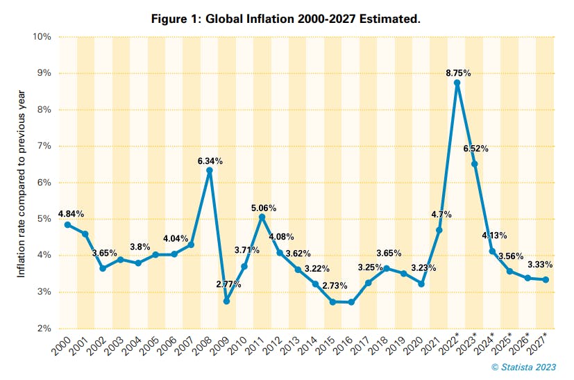
A sharp rise in inflation levels not seen for three decades (see figure 1), and a cost of living crisis in 2022, had ECR Retail Loss members asking ‘is inflation the reason for my increased Retail Loss/Shrink%?’

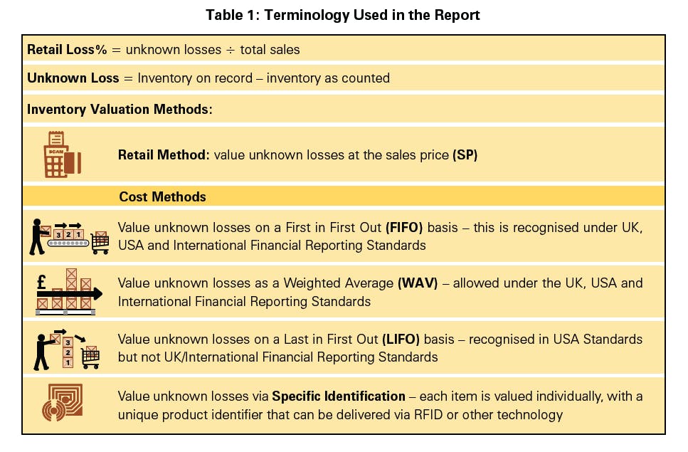
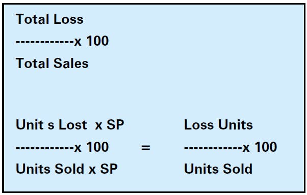
For the last 100 years, the Retail Loss% measure has been one of the most widely used and the most “emotional” metrics in retail. At its simplest it is either the units of unknown losses valued at either the cost of goods, typically the invoice value from the vendor, or the retail prices, divided by total sales value.

It is also commonly referred to as the ’Retail Shrink%‘ or just ‘Shrink%‘ however and in an attempt to promote clarity, ECR Retail Loss has encouraged retailers to adopt the use of Unknown Stock Loss as a more accurate term for describing any gap between the inventory expected at the time of an audit and the actual inventory found1 .

The question that we tackle here is whether the Retail Loss% (RL%), which we define as unknown inventory loss, is fit for purpose in difficult economic conditions, or indeed whether it is fit for purpose at any time.

In this report, the logic behind the Retail Loss% is tested using a simple two product model. This highlights the difficulties in identifying the effects at play in an inflationary environment. It is likely that the Retail Loss% masks what has actually been happening with losses at operational levels.

Following a detailed examination of the effects of inflation on the Retail Loss%, the final step in this report is to ask the critical question: Should the Retail Loss% be killed off?

Understanding Inflation

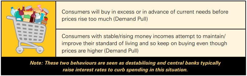
Classic periods of inflation in the 1950s, 1970s, around 1990 and around the 2008-2009 Financial Crisis arose because demand was greater than supply. As defined by Forbes: ‘Demand-pull inflation is when there is an increase in aggregate demand, and the supply remains the same or decreases. When supply cannot meet growing demand, prices for goods and services are pulled higher2 ’. To combat this, governments typically use interest rates to encourage saving rather than buying.

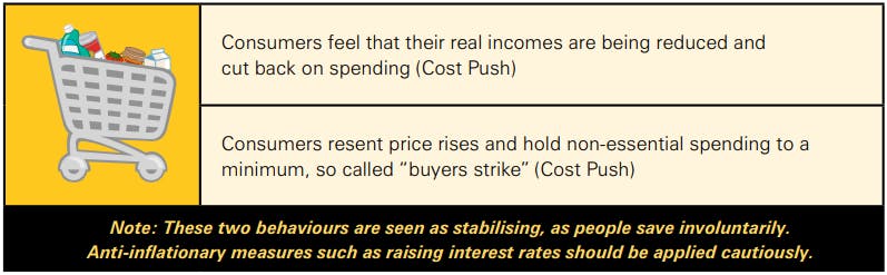
However, the current period of inflation has more in common with the rarer Cost-push form of inflation. This is where supply is lower than demand. ‘Cost-push inflation happens when there is a decline in the supply of goods and services and demand remains unchanged or even grows, driving prices and inflation higher3 .’ The problem is exacerbated when wages are depressed and in times of crisis.

Some writers have suggested that we are currently in a period of ‘Stagflation’, where ‘Stagflation is a period of stagnant economic growth accompanied by persistently high inflation and a sharp rise in unemployment.4 ’ However, unemployment is currently low but wages are failing to keep pace with inflation.

Consumer behaviour in this period of inflation is not entirely predictable but previous research in the field does allow us to understand what some of the behaviours might be, and how they directly affect the management of loss in retail.

Understanding Inflation and Consumer Buying Behaviour

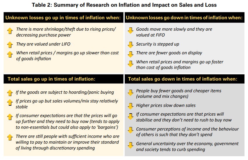
The research to date (detailed in Appendix 1) suggests that there is a spectrum of consumer behaviours in response to the expectation that inflation/prices are going to increase.

However, this economic model does not consider whether consumers may attempt to maintain their standard of living by what is called academically ‘unethical consumer behaviour’ – or more commonly known as fraud and theft.

Trade journals such as the The Grocer reported in 20225 that theft is a rapidly increasing trend. Kantar6 , Checkpoint7 and others report, about distorted patterns of unknown loss and total sales. They found consumers turn to discounters, own labels and ‘wonky veg’ in 2022. What we are seeing in 2022-23 is a reduction in spending coupled with an increase in retail loss for retailers.

Currently, there is a media trend to discuss saving money, not spending and being thrifty, and that wages are not keeping up with cost rises. Similarly, we know that there is social media learning around customer fraud in returns that rationalises theft and fraud as a necessity in a cost of living crisis that exacerbates previous online sharing on how to commit, say returns fraud.

In other words, retail loss prevention managers are fighting not just inflation but somewhat highly unpredictable patterns of behaviour in an uncertain economic policy environment fuelled by current discussions on various forms of media.

It seems likely then that a single KPI will not capture adequately the different consumer responses to expectations of inflation and price trends, and that perhaps a new approach is needed.

There are two immediate issues which may further complicate the picture:

• Sales are reliant on volume, price and assortment/mix.
• Unknown loss can be calculated in many ways, and is dependent again on the assortment of items included in the counts that allow for unknown loss to be calculated.

The basic question is whether RL% is going up because of inflation or because of some other factor(s).

In other words, is it the numbers and how they work together, or is it the behaviours that occur as a result of inflation, or is it the effects of the current cost of living crisis and not just inflation?

This exercise demonstrates the basic logic involved:

Let’s assume that RL% = 2% = 1/50, and then we apply some simple scenarios

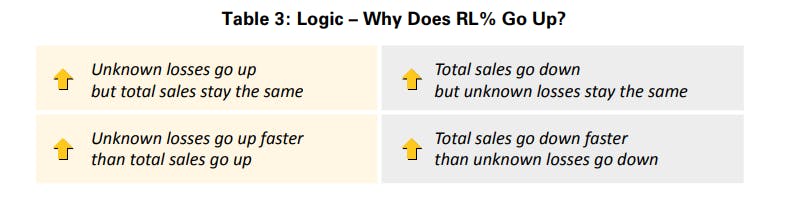
RL% goes up if total sales go down but there is no increase in the unknown loss.

e.g Sales decrease by 2%, RL% goes up by 4 bps (1/49 = 2.04%)

RL% goes up if unknown loss goes up but there is no increase in the total sales

e.g. Unknown loss goes up by 20% RL% goes up by 40bps (1.2/50 = 2.40%)

How likely is it that the entire 40bps rise is due to inflation?

RL% goes up if unknown loss value goes up faster than total sales value goes up, that is the rate of unknown loss increases faster than the rate of sales price increases then the RL% increases by 35bps

e.g. (1.2/51 = 2.35%)

For the RL% to stay at 2% when losses and sales value are increasing, implies a very high rate of inflation:

1.2/60 = 2% (which implies 17% inflation)

It seems that the effect of inflation on RL% might be to decrease, not increase the figure (See Appendix 1). This implies that RL% rises are not down to inflation but to volume and mix, and the reasons for the losses are probably derived from consumer behaviours.

To explore these observations more fully, a set of hypothetical scenarios was constructed based on the accounting for Retail Loss%.

Scenario Research

The detailed results can be found in Appendices 1-3.

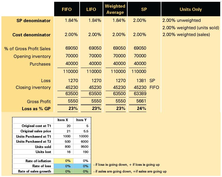
Using a simplified model to illustrate the effects of inflation and changing buying patterns, the effect of increasing rates of inflation and the effects of changes in consumer behaviours in times of inflation can be seen. There are two products only, X and Y. Following the logic example above, the RL% is 2% when there is no inflation, no change in unknown loss and no change in sales.

LESSON 1:

Changes in units are more important than valuation basis.

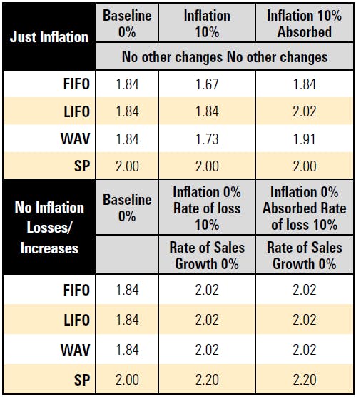
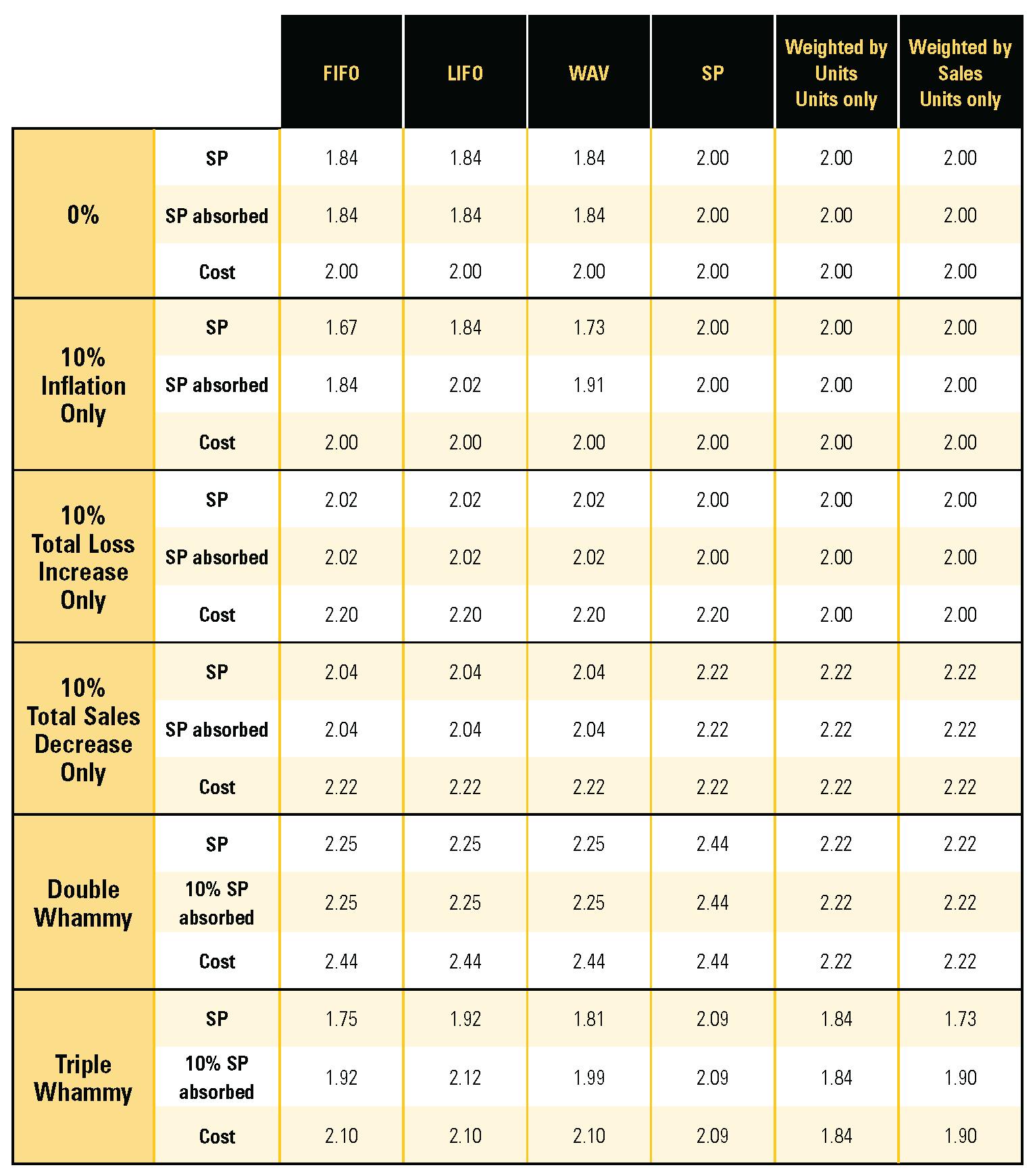
If all that changes is the rate of inflation and there are no changes in unknown losses relative to total sales, then RL% stays the same if sales price is used to value both unknown losses and total sales. It stays at 2% regardless of whether inflation goes up by 10% or down by 10%.

If unknown loss is valued at cost using FIFO or WAV, then the RL% does vary with inflation but this is because the units are now valued differently, not because of the rate of inflation itself. LIFO stays the same because it uses the most recent value, that is, it includes inflation while FIFO and WAV are based on uninflated cost prices. These differences can be up to 20bps. Interestingly, RL% goes down when a FIFO or WAV cost basis is used.

If the rate of inflation does not change but the number of units lost and/or the number of units sold change, then there is an effect on the RL% regardless of the cost basis on which the units are valued. These changes can be between 2bps and 20bps (See Lesson 2).

The logical conclusion is that UNITS are the most likely to reveal trends in Retail Loss in inflationary times than the RL% (see Lesson 2).

LESSON 2:

The effects of inflation on consumer behaviour are more important than the rate of inflation itself. The scenarios for changes in consumer behaviour are based on those seen in previous research (see Section 2).

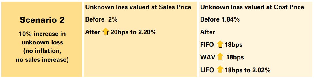
In inflationary times, there is a widely held belief that unknown loss will increase due to ‘unethical consumer behaviours’. Thus [Scenario 2] if unknown loss increases by 10% (that is, the number of units lost increases), but sales otherwise remain constant and inflation is zero, then RL% can increase by 20bps where SP is used to value units lost and by 18bps where a cost basis is used.

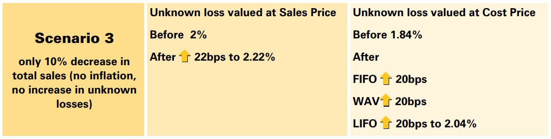
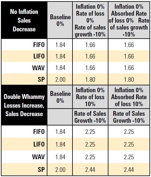
It is also likely in times of cost push inflation that sales will go down. If [Scenario 3] total sales units decrease by 10% but unknown losses stay the same and inflation is zero, then RL% can increase by as much as 22bps where SP is used to value units lost and by 20bps where a cost basis is used

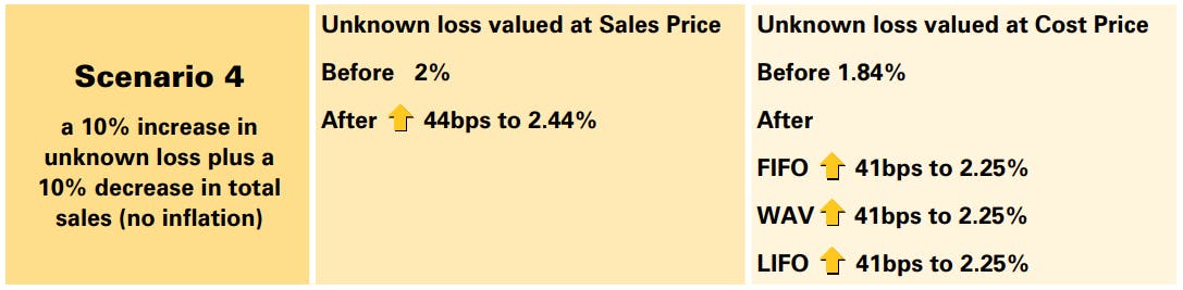
It is more likely that both unknown losses will go up and total sales will go down in times of inflation – a ‘double whammy’. Assuming [Scenario 4] that they both go up/down at the same rate of 10%, RL% can increase by as much as 44bps where SP is used to value units lost and by 41bps where a cost basis is used.

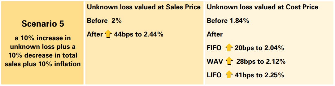
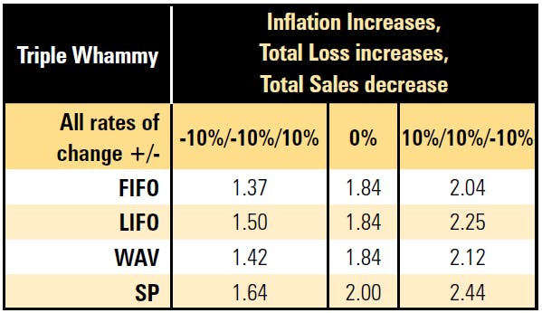
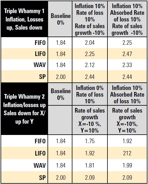
If [Scenario 5] we add in inflation at 10% to get a ‘triple whammy’ effect, then the only change is where FIFO, LIFO or WAV is used to value unknown loss. RL% can increase by 44bps where SP is used to value units lost and between 20bps and 41bps where a cost basis is used. However, as above, this appears to be due to the changes in units rather than the rate of inflation, which only has an effect when a different cost basis is used.

The problem here is that unknown losses and total sales will vary between SKUs and categories and so the effects could be hidden (See Lesson 3). However, if we look again at the real-life example in Box 1, looking at units lost per SKU, category or store would give a clearer picture of where the real issues lie in terms of understanding why losses are increasing.

LESSON 3:

Assortment and mix hide the effects of inflation and consumer behaviour in an overall RL% measure

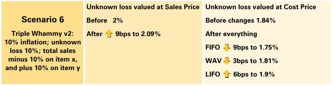
A more likely scenario [Scenario 6] is that more expensive goods will see higher losses and lower sales, but less expensive goods will see higher losses but also higher sales as consumers trade down.

By varying the effects on X and Y, where X sees higher losses but lower sales and Y sees higher losses and higher sales (all at 10%), the RL% shows much less variation than in the other scenarios. The effects are cancelling each other out, and hiding what is really happening at SKU, category and store level. In this ‘triple whammy 2’ scenario, RL% increases by 9bps where SP is used to value units lost and varies between 3bps and 9bps where a cost basis is used.

LESSON 4:

Absorption of inflation to help consumers can unfairly penalise loss prevention managers

The same scenarios were run again, this time assuming that the retailer absorbs all the higher costs of goods purchased and does not pass them through in higher retail prices. The detailed results of this scenario can be found in Appendix 3.

There are no changes to RL% when inflation is zero but unknown losses and/or total sales change.

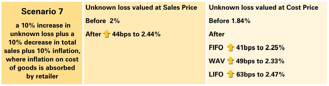
When [Scenario 7] inflation at 10% is included, the same patterns are observed but RL% can be as much as 44bps higher where SP is used to value units lost but this, as expected, is the same as with non-absorption. RL% varies between 9bps and 25bps where a cost basis is used and this is higher than for the non-absorption scenario. Hence, inflation leads to higher RL% when additional costs are absorbed depending on the cost basis used. This will also vary depending on whether the full or a partial cost increase is absorbed.

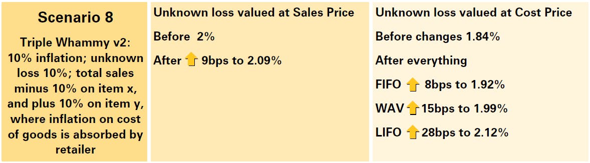
In the ‘triple whammy v2’ scenario [Scenario 8] the same pattern can be seen. The RL% is the same as for non-absorption if the SP is used to value losses but is higher than in the non-absorption scenario if a cost basis is used.

Therefore, loss prevention managers may be unfairly penalised for not meeting RL% targets where a cost basis is used to value losses, and will find it more difficult to untangle the causes of the increase. However, if SP is used to value losses, there are no new effects. The important factor appears to be changes in Units, not changes in inflation.

The overall conclusion, whether cost price rises are absorbed or not, is that the changes in units of losses and sales as a consequence of consumer behaviour are more significant than inflation in assessing why the RL% has increased or decreased.

One of the secondary considerations is that the RL% can mask different patterns of loss and sales for different items. Another is that inflation is unlikely to be the reason for significant increases in the RL%.

Financial ratios and KPIs in general, can suffer from similar problems to RL%. That is, they are very dependent on what is included in a particular cost or price, and the accounting policies adopted, by each business. Importantly, financial ratios and KPIs are measures that should be used to start conversations.

When setting measures, the Goodhart’s Law8 should always be kept in mind: ‘when a measure becomes a target, it ceases to be a good measure.’

The aim should be to have measures that allow managers to have those conversations about what is needed to meet changing consumer patterns of behaviour, and for executive directors to understand the impact of the loss on the business.

Alternative #1: Adopt Loss as a Percentage of Gross Margin as a Metric

One suggestion in the course of this study, is that loss as a percentage of gross margin could be examined. The main consideration is the effect of inflation on the closing inventory value, which will be higher than when inflation is stable.

This is good news for the business overall as the gross and operating margins will also be lower, and therefore taxation may be lower in times of inflation. However, there is a significant decrease in loss/gross margin when inflation is high. This could mislead management about the underlying issues involved.

An indicative set of figures was generated, using the same data as the test cases above. This shows that unknown loss as a percentage of gross margin where SP is used to value both losses and sales, is:

Base level (no inflation; no change in unknown loss; no change in total sales) Unknown Loss is 24% of gross margin.

Double whammy (no inflation; 10% increase in unknown loss; 10% increase in total sales) Unknown Loss is 24% of gross margin.

Inflation only (10% inflation; no increase in unknown loss or total sales) Unknown Loss is 12% of gross margin.

Triple whammy 2 (10%; 10% increase in unknown loss X&Y; 10% decrease in total sales X; 10% increase total sales Y) Unknown Loss is 13% of gross margin.

Although the measure loss/gross margin has the potential to be highly visual, it would be counterintuitive and volatile in times high inflation or deflation.

Alternative #2: Adopt Different Cost Bases

The model was used to calculate the RL% if like-for-like cost bases were used for the nominator and the denominator. This gives either:

Unknown loss valued at FIFO, WAV or LIFO/total cost of goods sold on same value of FIFO, WAV or LIFO

This gives an approximation of gross margin lost and is more closely aligned with cash flow. The problem is that cost of goods sold might include returns, discounts and other adjustments.

These calculations effectively strip out the costs/prices use, leaving a comparison of units, which is why the SP calculations column and the cost row are the same to within ±0.07.

The Results are shown in Appendix 3.

The key observations here are:

1. Using like for like cost bases smooth out variations seen under the different scenarios in Tests 1-5.
2. The variations between calculations are much smaller, usually within ±0.5%.
3. The most stable calculation is using total units lost/total units sold, without any valuation.

This suggests that unit based approach might be possible, in terms of measuring inventory management and cash flow management.

Alternative #3: Adopt Trending Analysis to Track the Rate of Unknown Loss Over Time

ECR Retail Loss carries out benchmarking between a number of retail members around rates of loss. An ongoing issue is that it is very difficult to compare retailers because each has a different way of classifying unknown loss. In other words, depending on what information can be extracted from data and finance systems in each retailer, different categories are included/excluded, and different losses are being tracked. It is also difficult to find a base level for the benchmarks, as calculation methods are being reset and refined on a regular basis.

Tracking whether unknown loss as a percentage is increasing or decreasing, and at what rate, has merit if the most stable calculations are concerned with units, rather than with costs or sales values. More detailed calculations could be carried out to identify which are low price and which are high price items, in order to isolate where the most impact is being felt.

A rate of change in unknown loss is also highly visual and can be represented by arrows, emojis or traffic lights for additional impact.

The most basic rate of change formula is:

Rate of change = (Change in quantity 1) / (Change in quantity 2)

This can be rewritten here as:

Rate of change in Unknown Loss over sales = (Change in Unknown Loss) / (Change in sales)

Hence:

((Unknown Loss units at Time 2 -Unknown Loss units at Time 1) / (Total units sold at Time 2 -Total units sold Time 1 )) X 100

Applying this to real-life anonymised data showing unknown loss in units, (Table 4), some interesting analysis begins to emerge:

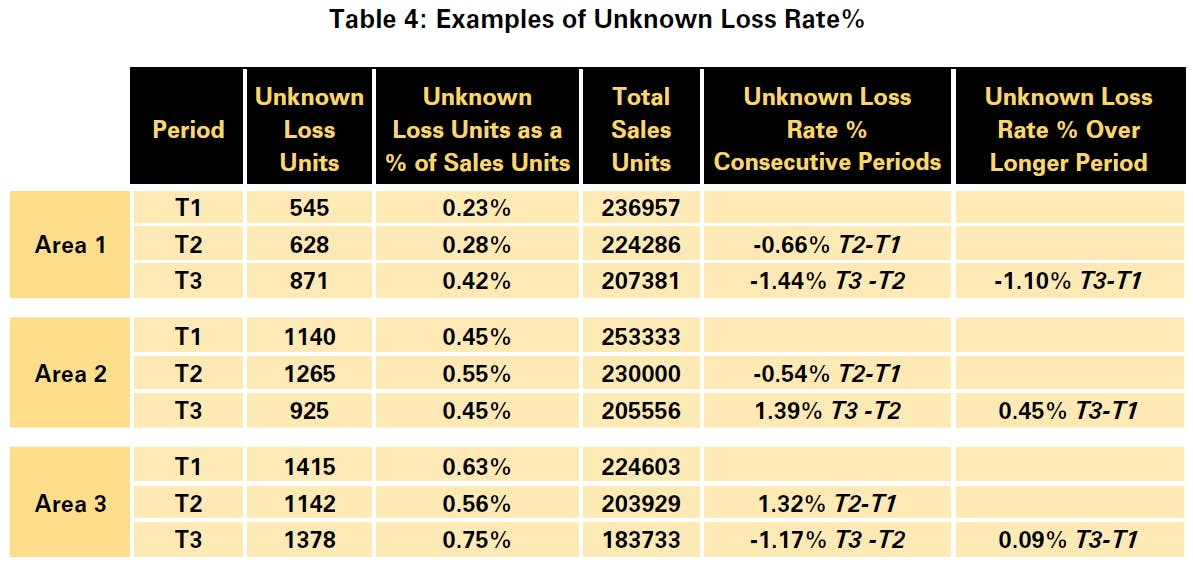
In Area 1, the unknown loss units as a% of sales units increases over the three periods, indicating that there is a problem needing serious attention. However, mitigation strategies would appear to be working, because a negative Unknown Loss Rate% implies that the rate of unknown loss is decreasing. This is because sales are decreasing more quickly than unknown loss is increasing, which represents a win for the loss manager.

In Area 2, the unknown loss units as a% of sales units increases then stabilises over the three periods, indicating that there is a problem but it might be under control. However, mitigation strategies may not be working, because the positive figure indicates that the Unknown Loss Rate% is increasing. Sales are decreasing faster than the unknown loss is decreasing, which is not a win for the loss manager.

In Area 3, the unknown loss units as a% of sales units fluctuates over the three periods, indicating that there is a problem needing serious attention. However, mitigation strategies would appear to be working, because the negative figure indicates that the Unknown Loss Rate% is decreasing. Unknown losses are increasing and sales are decreasing, but this is fluctuating: overall, just about a win for the loss manager over the longer period.

This suggests that a good alternative to the RL% is to look at a combination of unknown loss over sales in units as a percentage alongside the Unknown Loss Rate% for different time periods. This would be highly visual and could be demonstrated in time series analysis graphs.

An additional benefit of this approach is that it can enable greater sharing of the loss trends not only internally, but also externally between loss prevention managers working for different retailers. This will help with the constant question from the Board on retail losses, which is, how do we compare to other retailers?

Alternative #4: Adopt Specific Identification as a Valuation Method

The Corporate Finance Institute defines the specific identification method as follows9 :

• The specific identification method relates to inventory valuation, specifically keeping track of each specific item in inventory and assigning costs individually instead of grouping items together.
• It is useful and usable when a company is able to identify, mark, and track each item or unit in its inventory.
• The primary drawback to the specific identification method is that its use requires a definitive ability to easily and consistently identify all the individual items within a company’s inventory, track their cost, and produce them upon sale or the promise of sale.

Where item or unit has a Unique Produce Code (for example, using RFID), this can be used easily. At present, it is most often found where there are limited assortments of SKUs.

However, with Big Data, it should become easier to track inventory and losses, and to identify anomalies using machine learning or other AI techniques. This would not only assist loss managers in honing in on exceptional items, but also those forecasting, buying and pricing products for sale.

Implications, Limitations and Further Work

The analysis here suggests that unknown loss and total sales in UNITS are a better indicator of the issues involved because it is the consequences of inflation on consumer behaviour surrounding units lost or bought, not inflation itself, that are the problem. There are two important implications of the findings:

• That using RL% as a measure is insufficient to understand changes in consumer purchasing behaviours that might result in higher losses, and methods that focus more on units lost to provide an indicator of where loss prevention mitigations are needed at SKU, category, store and division levels.
• That using RL% as a target risks sub-optimal decisions being made by managers that reduce the RL% but that do not tackle the underlying issues of possible changing behaviours in times of high inflation.

The problem when RL% is used as both a measure and as a target is that Goodhart’s Law applies: when a measure becomes a target it ceases to be a good measure.

An aspirational goal would be for retailers to move towards specific identification of inventory and Big Data analysis of unknown retail loss. This would further allow analysis of which SKUs were problematic, as the losses could be valued and compared in greater detail.

However, a combination of unit based unknown loss percentages and unknown loss rate percentages over time offers a promising and highly visual alternative to the traditional RL%.

The findings of this study are limited because they use a simplified hypothetical model, which is supported by previous research into consumer behaviours and feedback from the loss prevention managers on their attempts to understand total retail losses in times of inflation.

Further work could include more extensive testing of in-store data or benchmarking.

Appendix 1

Appendix 1: Previous Research on Consumer Behaviour in Times of Inflation

The 1950s in the USA saw rising costs of goods as the country came out of WWII and experienced a surge in demand for consumer goods. The responses of consumers to increased prices in a study carried out by the Survey Research Centre10 at the University of Michigan concerning ‘The Origin and Effects of Economic Attitudes’, sound very familiar11. It is one of the first papers to look at the empirical evidence for consumer reactions to inflation. For example, the authors report that many responses state that ‘rising prices are bad for consumers; people cannot buy as much. The idea that when prices rise, wages tend to lag behind, also was expressed with some frequency’. Also, that ‘Most consumers associate stable or declining prices with “good buys,” sales and generous discounts rather than slack demand or bad times’. Overall, people felt that ‘rising prices retard their financial progress or tend to lower their standard of living’, and resented them accordingly.

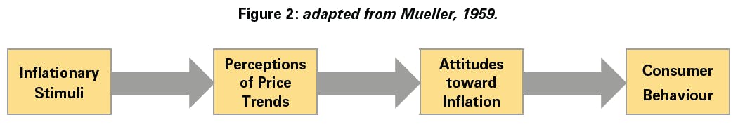
The 1959 study observes that ‘it is likely that some consumers will react in one way and some in another at any one time’. This is also the conclusion of more recent studies on inflation expectations and consumer behaviour. A more recent study from 201612 shows that ‘The average consumer tends to exhibit significantly varied micro-level expenditure behavioural patterns not readily observed at the macro- or aggregate-level expenditures.’ When prices are increasing, consumers buy fewer durable goods but maintain expenditure on non-durable goods and service expenditures. When there is a high level of uncertainty about the economic and political climate, consumer expenditure declines but in many varied ways. An Italian study13 found that expectations of higher inflation led to more spending on durable goods (that is, before prices got any higher) but also lowered purchasing power and spending where incomes were perceived to be effected (much as the 1959 study found). Here, household balance sheets explained spending behaviour.

Another interesting observation in the 1959 study was that consumers can learn behaviours, and this is also the finding of recent studies. In 2020, one study found that buying patterns following Covid-19 followed other major shocks in giving rise to panic buying and hoarding but they also found that people were learning behaviour from both mainstream and social media. A 2019 study in Portugal14 about behaviour in a recession found that there was also a learning journey that transformed people’s buying habits: ‘Besides switching to cheaper options, namely looking for private labels and national brand promotions, consumers revealed new strategies and new habits, such as i) more organization and planned behaviour; ii) going shopping more frequently; iii) reducing stocking behaviour, and iv) avoiding wasting.’ Currently, there is a media trend to discuss saving money, not spending and being thrifty, and that wages are not keeping up with cost rises. Similarly, we know that there is a social media learning around customer fraud in returns that rationalises theft and fraud as necessity in a cost of living crisis that exacerbates previous online sharing on how to commit, say returns fraud.

In other words, retail loss prevention managers are fighting not just inflation but somewhat unpredictable patterns of behaviour in an uncertain economic policy environment fuelled by current discussions on various forms of media. It seems likely then that a single KPI will not capture adequately the different consumer responses to expectations of inflation and price trends, and that perhaps a new approach is needed.

Appendix 2

Appendix 2: The Detailed Calculations from Each Scenario

The model used in the calculations is shown below.

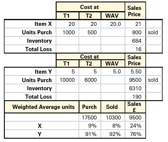
Experimental Results

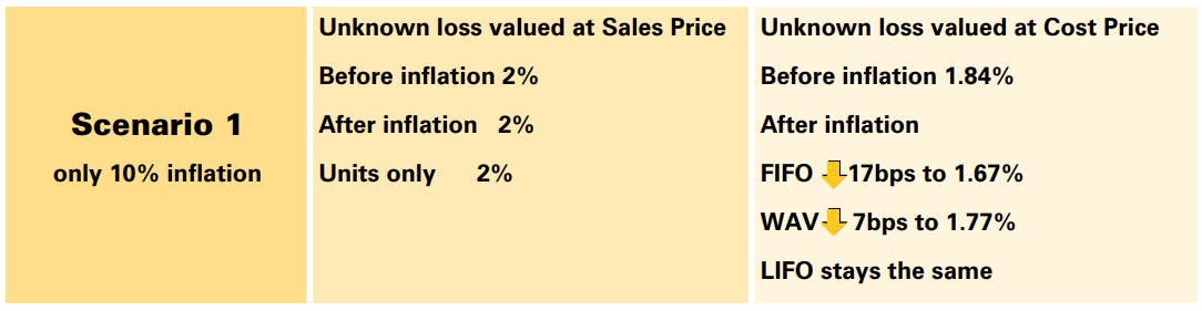
In Scenario 1, the rate of inflation was changed but the unit losses and unit sales stayed the same.

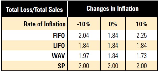
This shows that inflation only has an effect when the cost basis is FIFO or WAV.

This is logical, because if the same figure is used for both the nominator and the denominator, they will cancel out as follows:

This suggests that the number of units involved has a significant impact on the retail Loss%.

By definition, the FIFO cost stays the same for each change in the rate of inflation but the value of sales will increase. Therefore, the unknown loss increases more slowly than the total sales.

Three other patterns are noticeable:

1. The variation in Loss% across the rate of inflation changes is within a range of ±0.6.
2. The Loss% under FIFO and WAV valuations of unknown loss decrease as inflation goes up.
3. The Loss% under SP is higher than under the other methods.

In Scenario 2, only the unit losses changed. It assumes no inflation and no change in sales. For example, there was an increase in pilfering.

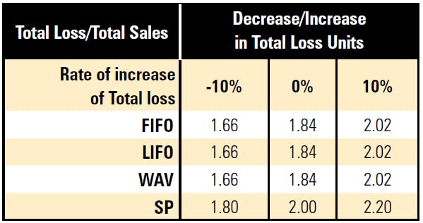
Here, the increase/decrease in the number of units lost has a marked effect, that has nothing to do with inflation.

Three other patterns are noticeable:

1. The variation in Loss% across the rate of loss changes is within a range of ±1.5.
2. The Loss% between FIFO, LIFO and WAV valuations of loss do not vary but SP valuations do have an effect.
3. The Loss% increases for all methods as the rate of loss goes up, and the figures using SP are higher than those using cost valuations.

In Scenario 3, only the unit sales changed. It assumes no inflation and no change in losses. For example, people buy less when times are hard.

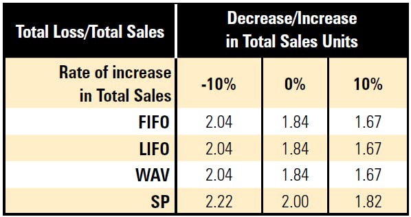
Again, the increase/decrease in the number of units lost has a marked effect, that has nothing to do with inflation.

Three other patterns are noticeable:

1. The variation in Loss% across the rate of loss changes is within a range of ±1.0.
2. The Loss% between FIFO, LIFO and WAV valuations of loss do not vary but SP valuations do have an effect.
3. The Loss% increases for all methods as the rate of sales go down, and the figures using SP are higher than those using cost valuations.

In Scenario 4, the ‘double whammy’ of unknown losses going up and total sales going down was examined. For example, people buying less and stealing more.

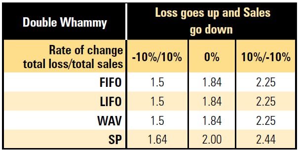
Once again, the increase/decrease in the number of units lost has a marked effect, that has nothing to do with inflation.

Similar noticeable patterns to those in Tests 1-3 can be seen. However, the new noticeable effect is that Loss% increases more rapidly and has a wider deviation of ±2.4.

In Scenario 5, the ‘triple whammy’ of the rate of inflation and unknown losses going up, but total sales going down for both items was tested.

As expected, there is a marked effect from unit changes (Tests 2-4) combined with a variation across the cost bases (Test 1).

The RL% increases even more rapidly and has a wider deviation of ±3.5.

In Scenario 6, the consumer behaviour is tested further. For the more expensive item, X, losses increase and sales go down. For the cheaper item, Y, losses increase but sales go up. For example, consumers buy less of the expensive item but want to keep up standards of living so shoplift the item rather than paying for it. The cheaper item is also stolen more but because it is cheaper, consumers switch to it from more expensive versions, thus increasing sales.

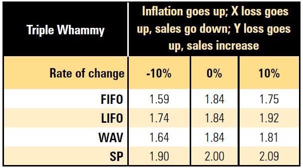
This is the most interesting test result, because the patterns of consumer behaviour offset each other. The RL% has less variation and the deviation is only ±0.9. The pattern of the Loss% is more erratic than in previous examples.

The problem is that this smaller change might be mistakenly attributed to inflation. Underneath, though, there are sizable losses at SKU level that would indicate significant operational issues that need to be tackled.

The tests were run again, but this time the calculations were adjusted so that the cost increases on purchases made by the retailer were absorbed and not passed onto customers [Scenario 7].

The indication here is that the absorption of inflation on costs by the retailer has the overall effect of increasing the RL%, because the total cost value will increase more quickly relative to total sales.

Appendix 3

Appendix 3: Detailed Comparison of Different Bases for Calculating RL%

The following table compares the differences in using a like-for-like cost basis for the calculation of the RL%. If loss is valued at FIFO and sales are valued at the purchase price rather than sales price then the effects of inflation absorption fall out of the equation.

End Notes

1. https://www.ecrloss.com/faq/retail-loss/how-is-Loss-or-shrinkage-measured???
2. https://www.forbes.com/advisor/investing/demand-pull-inflation/
3. https://www.thebalancemoney.com/what-is-cost-push-inflation-3306096
4. https://www.openaccessgovernment.org/bank-of-england-raising-interest-rates-inflation-finance-cost-of-living/147162/
5. https://www.thegrocer.co.uk/stores/shoplifting-on-the-rise-as-mounting-cost-of-living-bites/667686.article
6. https://www.kantar.com/uki/inspiration/fmcg/2022-wp-uk-grocery-price-inflation-up-again-as-shoppers-turn-to-wonky-fruitand-veg-to-cut-costs
7. https://checkpointsystems.com/blog/the-impact-of-inflation-on-shrinkage/
8. https://www.oxfordreference.com/display/10.1093/oiauthority.20110803095859655;jsessionid=E1C3EB3BEACC2A0DB6495FC786E2CE22.
9. https://corporatefinanceinstitute.com/resources/accounting/specific-identification-method/
10. Mueller, E. (1959). Consumer reactions to inflation. The Quarterly Journal of Economics, 73(2), 246-262.
11. The author looked at the reactions of consumers to rising prices and tested expectations of future price rises on buying behaviours (1951-1957)
12. Abaidoo, R. (2016). Inflation expectations, economic policy ambiguity and micro-level consumer behavior. Journal of Financial Economic Policy. 8(3), 377-395.
13. Rondinelli, C., & Zizza, R. (2020). Spend today or spend tomorrow? The role of inflation expectations in consumer behaviour. The Role of Inflation Expectations in Consumer Behaviour (April 27, 2020). Bank of Italy Temi di Discussione (Working Paper) No, 1276. Available at: https://ssrn.com/abstract=3612973
14. Sarmento, M., Marques, S., & Galan-Ladero, M. (2019). Consumption dynamics during recession and recovery: A learning journey. Journal of Retailing and Consumer Services, 50, 226-234.